Overview of model structure

    BIOME2 first calculates an optimal NPP and FPC for each of the woody plant types present in the grid cell. Competition between the woody plant types is then simulated by using the optimal NPP of each plant type as an index of competitiveness. The plant type with the highest NPP is selected as the dominant woody plant type.

    The optimal NPP and FPC of a specific plant type are found by running the coupled carbon and water flux models at a range of FPC values. Increasing FPC in- creases light absorption which increases photosynthesis and NPP. However, increasing FPC also increases evapotranspiration, which reduces soil moisture, creates drought stress, and decreases NPP. Thus, for a given environment and plant type, there is a certain FPC value for which NPP is maximal. In the model this maximum is located by examing the different NPP values simu- lated across the range of FPC values. The maximum NPP is selected as being the optimal NPP corresponding to an optimum value of FPC for a particular plant type. The calculated FPC for the woody plant type by itself then represents a maximum value for woody FPC. This value may be lowered by the inclusion of grasses.

    Competition between the dominant woody plant type and grasses is then simulated. A 'savanna' module cal- culates the whole-ecosystem NPP for various combina- tions of grass and woody FPCs. The optimal combina- tion of grass and woody plant types is then selected as being the FPC combination that maximizes whole-eco- system NPP.

    Model output consists of a quantitative vegetation state description in terms of PFTs present and their values of FPC and NPP. Finally, the predicted values of FPC for the different PFTs are grouped into vegetation classes for comparison with vegetation maps.

The carbon-flux model

    The carbon-flux model calculates the NPP of a specified plant type at specified FPC by a method conceptu- ally similar to the growth index approach of Specht (1981) and Nix (1981). 'Potential' NPP values are re- duced at low temperatures, and under water stress. The simplest equation for canopy photosynthesis assumes a linear relationship to absorbed photo- synthetically active radiation (PAR), which depends on foliage cover and reflectivity as well as on incident PAR (Monteith 1972, 1981; Linder 1985; Russell etal. 1989). These references provide empirical evidence that the relationship is indeed linear. Such a linear relationship can also be derived theoretically, by assuming that the maximum rates of photosynthesis for leaves at different depths in the canopy adjust (with response time < 1 month) according to their average PAR level, so as to give maximal daily net photosynthesis at that level (Field 1991; Sellers et al. 1992; Haxeltine & Prentice in press). This theory, fully developed in Haxeltine & Prentice (in press) shows how the total asimilation inte- grated over the canopy over a period of a month can be linear even though the instantaneous response of any given leaf follows the more familiar saturation curve shown in gas-exchange measurements. The simplest version of this theory has been implemented in the model presented here. We start by assuming a simple empirical relationship between instantaneous photosyn- thesis and PAR for single leaves (e.g. Landsberg 1986):

where A_n is the instantaneous net photosynthesis rate, is the quantum efficiency of gross photosynthesis at prescribed ambient CO₂, I is the instantaneous incident PAR flux, A_max is the maximum rate of photosynthesis, and R is the instantaneous rate of leaf respiration. We use the observation that R is approximately propor- tional to Amax (Hirose & Werger 1987; Givnish 1988; Field 1988):

R =aA_max

where a is an empirical parameter. Givnish (1988) compiled values of A_max and R for sun and shade-adapted plants. We derived a mean value for a = 0.08 from his data. Then, using the optimization constraint dAn/dAmax = 0 and integrating over a month (Haxeltine&Prentice in press) we can derive the relation:

where A_p is monthly potential photosynthesis, FPAR is the fraction of incoming PAR absorbed by the green vegetation, I_m is total monthly incident PAR, and a is a dimensionless factor that depends only on the fractional daylength (t_d) and the ratio of leaf respiration to photo synthetic capacity (a):

has a number of advantages for use at large scales. It gives a linear relationship of A_p to I, so the model does not have to consider the vertical structure of the canopy, only the total FPC. Maximum photosynthetic rates are implicit, and therefore do not need to be supplied as plant-type specific parameters. Monthly total PAR and average daylength are obtained from the same algorithm that calculates the net downward short-wave radiation flux for evapotranspiration. A full description of the equations used to calculate solar and net radiation and PAR may be found in Prentice et al. (1993a).

    Laboratory studies (Ehleringer & Bjorkman 1977) have established values of for C₃ and C₄ plants and their variation with temperature and CO₂. Ehleringer & Bjorkman (1977) measured a value of  for a C₃ plant at 13 °C of 0.07 mol(CO₂)/mol (photons). This fell to 0.04 at a temperature of 38°C. The for C4 plants does not vary greatly over this range of temperatures and was measured to be 0.054. However, values of  measured in field studies tend to be smaller by a factor of 2. Landsberg (1986) calculated a mean field value of  = 0.03. We used a conversion factor 0.03/0.054  0.55 to reduce the laboratory values to this level, while retaining the dependence of 0 on photosynthetic pathway and temperature.

    depends on the ratio of leaf respiration rate to photosynthetic capacity, which is a rather conservative quantity. Taking this ratio to be 0.08 (Givnish 1988) under present ambient CO2, we obtain for C3 plants at 20 °C (and 12 h day) a maximum efficiency for the conversion of absorbed PAR into carbon of ~ 2% on a molar basis. Including respiration costs (as described below) we obtain a maximum production efficiency of~1.2% (NPP(C) / absorbed PAR), or ~1.5 g(dry matter) per MJ of intercepted PAR.

    Monthly potential gross photosynthesis is reduced as follows according to environmental effects：

    where A_a is the actual monthly photosynthesis and the drought scalar is the ratio of actual to equilibrium evapotranspiration for the month as calculated by the water flux model. The monthly temperature scalar   is set to unity across a range of temperatures from T2 to T3. Below T2 the scalar  decreases linearly to at a temperature T1 and likewise above T3 the scalar decreases to zero at a temperature T4. This function describes the envelope of temperature  response curves for a range of species and climates: note a flat response over a broad range of temperatures,with photosynthesis declining only towards the extremes. We assume that vegetation in equilibrium with climate will show photosynthetic temperature responses that are well adapted within the optimum range (T2-T3）defined for the plant type . T3 and T4 were set at 45°C and 60°C respectively for all plant types, i.e. values greater than the highest mean monthly tempeture encountered.

   FPC is defined as the fraction of ground covered by foliage vertically above. FPC directly measures the ability of the canopy to intercept radiation. We therefore simply equate FPAR to FPC. The phenology routine sums daily FPC values type to produce monthly averages of FPAR.

   Over a wide range of plant types, whole-plant respiration costs are typically 30-70% of gross primary production. We model ration as 40% of potential photosynthesis.We assume that as drought stress and temperature stress increases(reducing gross primary production),respiration costs stay fixed. This fixed. This means that respiration costs higher proportion of the actual gross primary production as environmental stress increases,thus:

NPP = A_a -0.4A_p

    NPP is calculated each month and summed for the year. When leaves are absent respiration costs continue, but at 1/3 of the rate implied by NPP = A_a -0.4A_p

The water-flux model

    Water availability is calculated by a two-layer soil hydrology model derived from that of Neilson (1995). The purpose of the water-flux model is to provide meas- ures of drought stress for use by the carbon-flux model, so the appropriate level of complexity is the simplest needed to provide an effective measure of the drought stress experienced by different plant types. The water- flux model uses a daily timestep, interpolating monthly climate data to yield quasi-daily values. A daily time step is used only to simplify the numerical calculations. The results are aggregated to a monthly time step and fed back to the carbon-flux model.

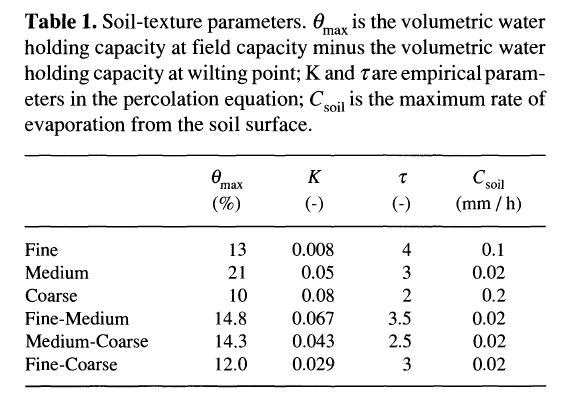
    The soil is described by two layers at depths 0-0.5m and 0.5-1.5m. Available water capacity(AWC) for each layer is defined as the difference between field capacity and wilting point for the relevant soil texture. In texture-contrast soils AWC has different values for the two layers. Percolation from the upper layer to the lower layer is calculated using an empirical equation adaped from Neilson. Percolation depends on soil teature. No runoff is allowed from the lower layer.Percolation ceases when the lower layer reaches field capacity.Runoff from the upper layer occurs when this layer reaches field capacity. The percalation formula is:

where Perc is the daily percolation(mm) from the upper to the lower soil layer,K and are empirical constants dependent on soil texture, d1 is the depth of the top soil layer(mm), is the volumertric soil moisture in the upper soil layer(m3·m-3)，and  and  are the volumetric soil moisture values at wilting point and field capacity respectively.

    The instantaneous evapotranspriation(E) is calculated daily as the lesser of an instantaneous supply(S) and demand(d) function:

E=min（S，D）

    E=min（S，D） is integrated analytically over the 24-h period (Federer 1982; Prentice et al. 1993a). The demand func- tion is derived from the theory of equilibrium evapotranspiration (Jarvis & MacNaughton 1986). Ac- cording this theory, when soil moisture is not limiting, the (large-scale) evapotranspiration rate is determined by the energy supply for evaporation (the equilibrium evapotranspiration rate). We use this equilibrium rate as the (instantaneous) demand:

where s is the rate of increase of the saturated vapour pressure with temperature (Pa K^-1);is the psychrometer constant (Pa K-1); and L is the latent heat of vaporization of water (J kg-1). Tables are used to take account of the weak dependence of  and L on temperature, and s is calculated as a function of temperature using the rela- tionship given in Prentice et al. (1993a). Rn is the instan- taneous net radiation flux (W m-2) calculated from lati- tude, temperature and sunshine hours using an algo- rithm fully described in Prentice et al. (1993a).

    The supply rate is calculated as a function of avail- able soil moisture (Prentice et al. 1993a). However the land surface of the grid cell is now divided up into a bare soil fraction and the fractional cover (FPC) of each plant type present. The supply function is specific to each plant type present and is a function of the effective soil moisture experienced by that type:

S_i = Ci Wri

where Si is the supply function for type i , Wri is the average soil moisture in the root zone of type i (expressed as a fraction of the maximum possible soil moisture in the root zone), and Ci is the maximum possible rate of evapotranspiration from plant type i. The effective (plant-available) soil moisture is calculated from an estimate of the relative proportion of roots in each soil layer such that:

Wri =ZiW1 + (1-Zi)W2

where Wri is the available soil moisture in the rooting zone of plant type i and W1 and W2 are the total extractable water contents of the upper and lower soil layers respectively, as calculated from Eq. 8. Zi is the fraction of the roots of plant type i that are in the upper soil layer. A mean value of Ci = 1.0 mm.h^-1 was assumed for all plant types (Federer 1982). 

    Evapotranspiration from bare soil is calculated in an analagous way: 

S_soil = C_soil W₁

where S_soil  is the (supply limited) rate of soil evapora- tion, and C_soil  is the maximum rate of evaporation from the soil surface under saturated conditions. C_soil  depends on soil texture (Table 1). Each day, the model calculates a transpiration rate Ei for each plant type i, and an evaporation rate E_soil  for the evaporation rate from the soil surface. Following Abramopoulos et al. (1988), we calculate total evapo- transpiration from the land surface as the sum of the components from each vegetative layer and that from the bare soil fraction. The phenology routine updates FPC at a daily time step. The FPC of each plant type is by definition directly equivalent to its ground cover fraction. Thus the actual evapotranspiration per unit area of land surface is found by multiplying each Ei by the ground cover fraction (fi) for that plant type. So for two plant types, the total evapotranspiration rate E_total is given by:

E_total =f_iE1 +f2E2 + (1 -f1 -f2)E_soil 

    The soil moisture stores are updated each day using the daily percolation (Perc), quasi-daily rainfall (Rain) and the calculated evapotranspiration rates:

where W₁ⁿ⁺¹ and W₂ⁿ⁺¹ are the updated extractable soil water contents for the current timestep; W1 and W2 are the values from the previous timestep, all evapotranspi- ration rates being evaluated at these soil-moisture val- ues; d₁ and d₂ are the depths of the upper and lower soil layers respectively; are the volumetric water-holding capacities () of the upper and lower soil layers respectively. are the rates of extraction of water by plant type i from the upper and lower soil layers. The relative rate at which a given plant type extracts water from either soil layer is a function of its rooting characteristics as expressed in the parameter Z_i. The rates of water extraction by plant type i from the two soil layers are thus:

    The climate data used to force the model have monthly resolution, so the maximum resolution of model output is monthly. The water balance model therefore supplies a plant type-specific drought scalar to the carbon balance model at a monthly timestep.The drought scalar is:

    where Ei is monthly actual evapotranspiration and D is monthly equilibrium evapotranspiration. The carbon and water flux models are thus coupled by their co-dependence on FPC and by the influence of the drought saclar  on the rate of photosynthesis.

Plant types

    For Australia we assumed that just two woody plant types (evergreen and drought-deciduous) and two grass plant types (C3 and C4) can occur, and that these could in principle be found anywhere. We aimed for the mini- mum of plant type-specific parameters (Table 3). Shrubs were not modelled explicitly; woody plant types were categorized as shrubs or trees after the main analysis.

    The most important difference between woody and grass plant types in the model is in their rooting strate- gies. Generally, grasses have most of their roots in the upper soil layer (ca. 2 - 60 cm), whilst woody plant roots have access to water resources in both the upper and lower soil layer.In BIOME2, grass roots extract water almost entirely from the upper (0-0.5m)soil layer while woody plant roots extract water from both upper and loewe soil layers. This formulation allows the modedl to simulate competition for water resources between grass and woody plant types.

     Evergreen trees are assumed to maintain a constant FPC through the year. A simple phenology algorithm is used for drought-deciduous trees and grasses: FPC is reduced to zero whenever the drought scalar falls below a threshold value (Table 3). This value was estimated as the maximum drought stress allowing positive net photosynthesis. The two woody plant types were assigned different temperature responses because drought-deciduous trees are exclusively tropical (frost- or chillsensitive) and have a high temperature optimum for photosynthesis, whereas evergreens include tropical and temperate types with a wide range of photosynthetic temperature optima (Hill et al. 1988). In the model the equatorward spread of evergreens is limited by their relative uncompetiveness (due to high dry-season respiration losses) in the strongly summer-rain climate of northern Australia, while the poleward spread of drought-deciduous trees is limited by lower temperatures that progressively favour evergreens.

    The choice of a C4 or C3 grass type is made basis of mean monthly temperature. Above grasses have a higher quantum efficiency than (Long & Hutchin 1991). So in the model, when monthly temperature is 30 ?C or greater, the grass selected for that month is C4. The model thus and C3 grasses to co-occur but during different the growing season, in agreement with observations Australia (Groves & Williams 1981; Hattersley and elsewhere (Ehleringer 1978; Fowler 1981; Ehleringer & Monson

Predicting combinations of grass and woody plant types

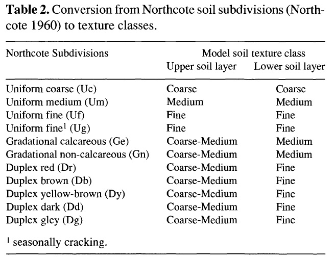
    Competition between woody plants and grasses is modelled using a two-layer soil model with a texture- dependent calculation for water percolation. The hy- drological properties of each layer are prescribed from soil texture. The optimal combination of woody plants and grasses is found by comparing total NPP for differ- ent combinations of the dominant woody plant type with the appropriate (seasonally varying) grass plant type. All combinations of woody and grass FPC summing to 100 % or less are tried, at steps of 10 % FPC (with additional values at 5 % and 15 %). The combined grass and woody FPC may not be more than 100 %.