Quoted from: https://ccmc.gsfc.nasa.gov/models/models_at_glance.php 

Model Description
This is an exospheric model of the solar wind with only protons and electrons (we defer the inclusion of heavy ions to upcoming versions of the code), with a non-monotonic total potential for the protons and with a Lorentzian (kappa) velocity distribution function (VDF) for the electrons. This code is developed for the coronal holes.

Exospheric kinetic models assume that there is a sharp level called the exobase, separating a collision dominated region (where a fluid approximation is valid) from a region fully collisionless. In fact, there is a transition region where collisions between particles become less and less numerous when the distance to the Sun increases. Click here to read more about the basics of the exospheric kinetic models.

Model Input

• Radial Distance of the Exobase: The radial distance of the exobase in solar radii. It must be located between 1.1 and 5 because the model has been developed for the coronal holes where the number densities are lower than in equatorial streamers. In equatorial streamers, the exobase level is located at a larger distance from the Sun and the total potential of the protons is a momotonically decreasing function of the radial distance (which means that the repulsive electrostatic forces is larger than the attractive gravitational force at every radial distance above the exobase).
• Electron Temperature at Exobase: The temperature of the electrons at the exobase in K. This temperature is usually observed to be between 800000 K and 2000000 K.
• Proton Temperature at Exobase: The temperature of the protons at the exobase in K. This temperature is usually observed to be between 1000000 K and 2000000 K.
• Kappa Index Value: The values of the kappa index of the electrons VDF at the exobase. This value ranges from 2 to 1000 (~ inifinity, the Maxwellian case). However, when the exobase is located low in the solar corona, a certain amount of suprathermal electrons is necessary in order to accelerate the solar wind to large velocities (> 500 km/s). The characteristics of the fast solar wind originating from the coronal holes are obtained with kappa between 2.5 and 3.0, also corresponding to typical values obtained by fitting the electrons VDF of the solar wind with Kappa distributions (see Maksimovic, Pierrard & Riley, Geophys. Res. Let., 24, 9, 1151-1154, 1997).
• Max Radial Distance: The last radial distance (in solar radii) where the program calculates the moments of the electrons and of the protons VDFs of the solar wind.

Model Output

• G_p: the total normalized potential of the protons (unitless)
• PHI: the electrostatic potential (in Volts)
• N_e: the number density of electrons (in 106m-3
• N_p: the number density of protons (in 106m-3
• F_e: the flux of electrons (in 1012m-2s-1)
• F_p: the flux of protons (in 1012m-2s-1)
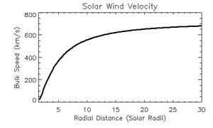
• V_e: the bulk velocity of the solar wind electrons (in kms-1)
• V_p: the bulk velocity of the solar wind protons (in kms-1)

References and relevant publications
H.Lamy, V.Pierrard, M.Maksimovic and J.F.Lemaire, A Kinetic Exospheric Model Of the Solar Wind With a Nonmonotonic Potential Energy For the Protons, J. Geophys. Res., 108, 1047, 2003.

Relevant links
IASB
Full Model Description Document

CCMC Contact(s)
Masha Kuznetsova
301-286-9571