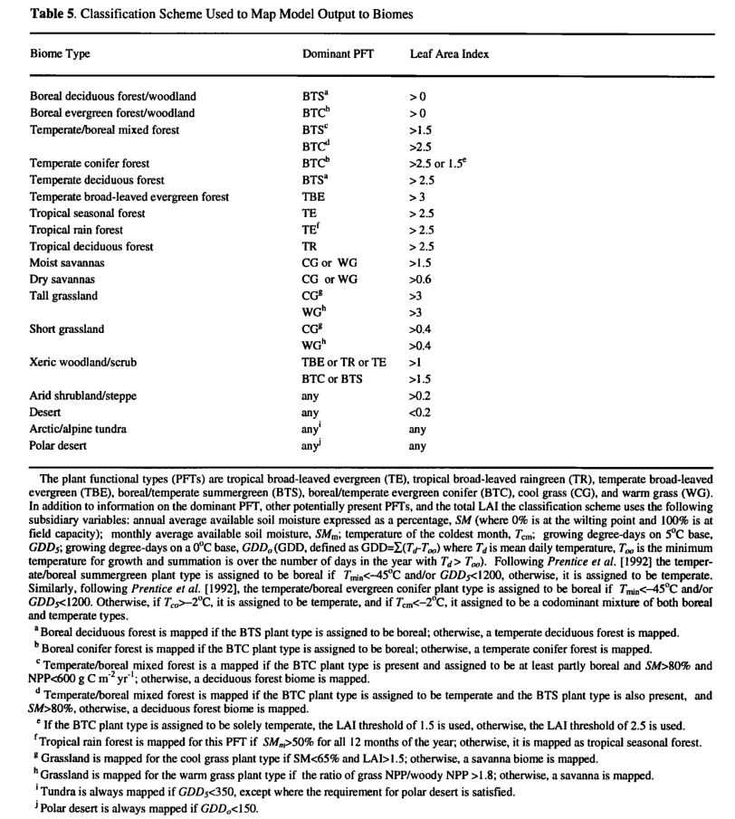
The essential model logic is as follows. First, BIOME3 selects from a global set of plant functional types (PFTs) the subset which may potentially be present in a particular grid cell on the basis of a small number of ecophysiological constraints. Using a coupled carbon and water flux model and an optimization algorithm, BIOME3 then calculates the maximum sustainable leaf area index (LAI) and net primary production (NPP) for each PFT. Competi­tion among PFTs is simulated by using the optimal NPP of each PFT as an index of competitiveness. A semi-empirical rule de­signed to capture the opposing effects of succession driven by light competition and natural disturbance by fire excludes grasses as a dominant PFT if soil conditions are too wet. The PFT with the highest NPP is selected as the dominant plant type, except where grasses have been excluded. Model output consists of a quantita­tive vegetation state description in terms of the dominant PFT, secondary PFTs present, and the total LAI and NPF for the ecosystem. This output can be classified into biome types for comparison with vegetation maps.

The model is driven by monthly climate data. Model outputs are therefore at a monthly or yearly time step. Photosynthesis and canopy conductance are calculated at a monthly time step. The water balance and phenology models, however, work on a daily time step for reasons of numerical stability. Monthly temperature and cloudiness data are interpolated linearly between midmonths to yield quasi-daily values. Values for canopy conductance are calculated daily and then averaged to produce values for averaged midmonth days Output from the water balance and phenology submodels are averaged to provide monthly average values for use by the photosynthesis and canopy conductance submodels.

1.Selection of PotentiaUy Present Plant Types

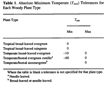
Prentice et al [1992] summarized the different cold tolerance mechanisms employed by woody plant forms and demonstrated the importance of minimum temperatures in determining the world distributions of different types of woody plants. Following Pren­tice et al. [1992], each of the values in the first data column of Table 1 represents an approximate point of failure for a different cold tolerance mechanism, based mainly on observations summa­rized by Woodward [1987], BIOME3 controls the distribution of the plant functional types employing these different mechanisms using data on absolute minimum temperature rather that by using an approximate relationship to mean coldest-month temperatures as in the model of Prentice et al. [1992]. The absolute minimum temperature tolerances given in Table 1 are the same as those giv­en in Table 2 of Prentice et al. [1992] except for the temperate broad-leaved evergreen plant type (as it has no direct equivalent in the work of Prentice etal. [1992]) for which a value was estimated from Woodward [1987]. Chilling requirements are minimally rep­resented by requiring an absolute minimum temperature below 0°C for temperate and boreal PFTs (Table 1). Prentice et al.[1992] distinguished temperate summergreen trees from boreal summergreen trees and temperate evergreen (coniferous) trees from boreal evergreen (coniferous) trees. In BIOME3 these dis­tinctions are made only at the mapping stage, because in principle they do not affect the deciduous/evergreen competition. Applica­tion of these temperature limits results in the selection of between one and three potentially dominant woody PFTs.

2. Coupled Carbon and Water Flux Model

Photosynthesis. Photosynthesis is calculated as a function of absorbed photosynthetically active radiation (APAR), tempera­ture, atmospheric C 〇 2 concentration, day length, and canopy conductance. Calculations are made for an averaged midmonth day and multiplied by the number of days in the month. APAR is calculated from the net photosynthetically active radiation (PAR) multiplied by the fraction of incoming PAR intercepted by green vegetation (FPAR). FPAR is calculated from the projected leaf area index (LAI) using Beer's law [Monsi and Saeki, 1953]:

where k is an extinction coefficient. Measurements of k indicate that it varies considerably among different species of plant and that it is also dependant on sun angle [Larcher, 1983]. Here we use an average value of k (Table 2) appropriate for modeling photosyn­ thesis at large scales [Woodward, 1987]. The net PAR flux is calculated from latitude, temperature, and sunshine hours data us­ing an algorithm fully described in the appendix. Canopy conductance is calculated as a function of potential photosynthesis rate and water stress through coupling with the water flux model. Water stress is assumed to reduce photosynthesis through a reduc­tion in canopy conductance. The mechanism of this reduction is not treated explicitly.

The photosynthesis scheme is based upon the Farquhar photo­ synthesis model as simplified by Collatz et al. [1991]. However, instead of prescribing values for the Rubisco capacity (Vm), we use an optimization algorithm to predict, for each month, the value of Vm that gives the maximum (non-water-stressed) daily rate of net photosynthesis. This algorithm is based upon very extensive evi­dence, summarized by Haxeltine and Prentice [1996], for the hypothesis that the N content and Rubisco activity of leaves vary both seasonally and with canopy position in such a way as to max­imize net photosynthesis. Here leaf nitrogen content is not modeled explicitly; instead, the optimization is carried out directly on the Rubisco activity of leaves. The optimization depends on the fact that both the maximum rate of gross photosynthesis and the leaf respiration rate increase with the activity of photosynthetic enzymes (most importantly Rubisco) in the chloroplasts. This re­sults in a trade-off: a high net photosynthesis rate at high PAR can be achieved by having a high Rubisco activity, but this also implies a low, or negative, net photosynthesis rate at low PAR. Thus, for any PAR level there is an optimal photosynthetic enzyme activity that produces maximum net photosynthesis.

The resulting scheme has the important feature that it predicts lightuse efficiencies that are independent of PAR. Haxeltine and Prentice [1996] showed that this scheme estimates lightuse effi­ciencies consistent with those measured in crop ecosystems but up to double those measured in natural ecosystems. They hypothe­ sized that this is because lightuse efficiencies and photosynthesis rates are reduced in natural ecosystems by temperature, water, and nutrient stresses.

Here we summarize the photosynthesis scheme, for which Hax­eltine and Prentice [1996] give a full rationale. Daily net photo­synthesis is calculated using a standard nonrectangular hyperbola formulation, which gives a gradual transition between two limiting rates: J e , describing the response of photosynthesis to APAR; and Jc，describing the Rubisco limited rate of photosynthesis [Collatz etal., 1991; Haxeltine and Prentice, 1996]

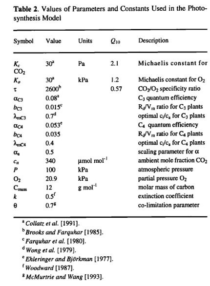
where A_nd is the daily net photosynthesis (g C d^-1m^-2) and R_d is the daily leaf respiration rate (g C d^-1m^-2). APAR is the daily total absorbed PAR (mol d^-1m^-2), and α_c3 is the intrinsic quantum effi­ciency for CO₂ uptake as measured in laboratory studies. The empirical parameter aa accounts for reductions in PAR utilization efficiencies in natural ecosystems, and is assigned a value of 0.5 based on data summarized by Landsberg [1986] on quantum effi­ciencies from field and laboratory measurements. Cmass is the molar mass of carbon，and pi is the internal partial pressure of CO₂ ,given by

where p_a is the ambient partial pressure of CO₂ and λ is a parameter. Many observations have shown that, for C₃ species under non-water-stressed conditions, stomata respond in a way that maintains a constant ratio of intercellular (p_i) to ambient (p_α)CO₂ partial pressure of 0.6-0.8 [Wong et al., 1979; Long and Hutchiny 1991]. We therefore set A, equal to a maximum value(λ_mC3 = 0.7 ) under non-water-stressed conditions, Γ_* is the CO₂  compensation point given by

where [O₂] is the partial pressure of oxygen. K_c, K_o , and τ are kinetic parameters whose temperature dependence is modeled us­ing a Q₁₀ relationship. The empirical parameter θ describes the transition between the two limiting rates J_E and J_C  and may be determined experimentally. The inhibition function  Φ_tc3 models the effect of low temperatures on C₃ photosynthesis:

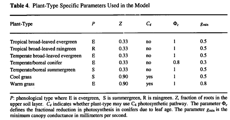
where Tc is the monthly temperature (in degrees Celsius). The function was adjusted so as to approximate the response of C3 photosynthesis to low temperatures [Berry and Bjorkman, 1980]. Oc is a PFT specific parameter (Table 4) to account for the obser­ vation that maximum rates of photosynthesis for conifer needles decrease with increasing needle age. Leaf respiration (Rd in g C d^-1m^-2) was scaled to Vm as

where bc3= 0.015 [Farquhar et ai, 1980]. The values of all pa­rameters and constants used in the photosynthesis model are given in Table 2.

The model calculates the value of Vm which gives the maximumdaily rate of net photosynthesis. This optimal value for Vm is cal­culated by optimizing ( 2 ) using the constraint  result­ing in the following equation for Vm (g C d^-1m^-2):

where dt is the day length in hours, calculated as described in the appendix.

A model for C₄ photosynthesis was adapted from Collatz et al,[1992] using the same optimization procedure. For C 4 photosyn­thesis the functions Cl_c3 and C2_C3 are replaced by C1 〇 a and C 2C4 which are calculated as

where  α_C4 is the intrinsic quantum efficiency for C₄ photosynthe­sis, and Φ_pi and  Φ_TC4 are scalars which reduce the  C₄  photosyn­thesis rate below its optimal value. Φ_pi captures the effect of reduced pi on C₄ photosynthesis:

where λ_mC4 is the value of X which C₄ plants maintain under non­ water-stressed conditions.  Φ_TC4 accounts for the approximate re­sponse of C₄ plants to extreme temperatures, following Collatz et.al [1992]:

Leaf respiration costs are calculated as in (10) but with the pa­rameter b_C3 replaced by b_C4. The value of b_C4 was scaled so as to give leaf respiration costs for b_C4 photosynthesis similar to those predicted for C₃ photosynthesis. An optimal value of Vm is calcu­lated from ( 11 ) using the appropriate functions and parameter values for C₄ photosynthesis [Haxeltine and Prentice, 1996]. The values of all parameters used in the C₄ photosynthesis model are listed in Table 2.

With a plentiful water supply this scheme gives C₄ photosyn­thesis rates that are lower than C₃ rates at temperatures <20°C;above this temperature, C₄ rates are higher. Water stress tends to have a greater effect on the modeled C₃ photosynthesis rate than on the C₄ rate; thus water stress lowers the temperature at which the C₄ photosynthesis rate exceeds the C₃ rate.

The photosynthesis rate may be related to canopy conductance through the diffusion gradient in CO₂ concentration implied by the difference in CO₂ concentration between the atmosphere and in­tercellular air spaces. Expressing this relationship in terms of the total daytime net photosynthesis A_dt gives

where g_c is the average daytime canopy conductance. The param­eter gmin is a PFT specific minimum canopy conductance, which accounts for plant water loss not directly associated with photo­synthesis (e.g. cuticular transpiration). The variable ca is the ambient mole fraction of CO₂ (Pn=Pxc_a, where P is atmospheric pressure). The factor of 1.6 accounts for the difference in the dif­fusion coefficients of CO₂ and water vapor. A_dt is given by

Equation (18) may be rearranged to calculate a value for g_c:

Use of the maximum non-water-stressed value for λ(λmc3 for C3 photosynthesis) allows the calculation of the maximum poten­tial photosynthesis rate and maximum potential canopy conduc­tance (g_p) realizable under non-water-stressed conditions

Water stress results in a lower canopy conductance. In which case the water balance calculation provides a value for the actual(water-limited) canopy conductance; (18) is then solved as a si­multaneous equation with ( 2 ) (using a bisection method) to obtain the water-limited values of A_nd and λ. Evapotranspiration. The actual evapotranspiration (AET) is calculated at a daily time step as the minimum of a supply function S and a non-water-stressed evapotranspiration rate D:

D is calculated as a function of the potential canopy conductance (g_p) using a simple planetary boundary layer parameterization adapted from Monteith [1995]

where E_q is the daily total equilibrium evapotranspiration calcu­lated from latitude, temperature and sunshine hours data as described in the appendix. The parameters am and gm are empirical parameters with am = 1.4 and gm = 5 following Monteith [1995]. The variable gp is the non-water-stressed potential canopy con­ductance predicted by the photosynthesis model. D gives the evapotranspiration rate which the vegetation achieves when the supply of moisture from the soil is not limiting.

Following Prentice etal. [1993], the supply function is propor­tional to the soil moisture in the rooting zone (W_r):

where  E_max is the maximum daily transpiration rate possible under well watered conditions, assigned a value of 5 mm d^-1 based on on differences in the modeKs ability to predict different vegetation classes and, using a subjective scale, can be used to assess the predictive ability o f the model.  Monserud [1990] suggested that values <0.4 be considered poor or very poor, values 0.4-0.55 be considered fair, values 0 55-0 7 be considered good, values 0 7-0.85 be considered very good and values >0.85 be considered excellent. A generalized form of the kappa statistic  [Prentice et al.t 1992] can be used in a similar way to examine the agreement between the two maps at spatial scales larger than the grid size. Adjacent grid cells are grouped into blocks and the proportions of different classes within each block are calculated. The overall agreement between maps is then based on the similarity between the proportions of different classes found within the blocks.

The overall kappa statistic reveals a fair agreement (0.53) be­tween the maps at a 0.5° block size and a good agreement (0.58) at a larger 2.5° block size.  M odel predictions thus show a better agreement with the vegetation map at larger scales. This is to be expected because both the soils and vegetation data sets are largely composed of data originally digitized at a 1° resolution rather than the 0.5° resolution used for this study, and the 0.5° climate data set was produced by interpolation between clim ate stations with a spacing often considerably more than 0.5°. Individual kappa sta­tistics for each biome are shown in Table 6 for block sizes of 0,5° and 2.5°. They reveal differences in the models performance for different vegetation classes.

The predicted extents of the forest and woodland classes gen­erally show a fair to good agreement with the vegetation map. Exceptions are the temperate conifer, tropical deciduous forests, and xeric woodlands/scrub classes. The predicted distribution of temperate conifer forest is in very poor agreement with the map. The predicted extent of xeric woodlands/scrub biome shows a poor agreement with the map on the basis o f the kappa statistic. How­ever, the model correctly predicts areas of xeric woodlands/scrub in southwestern Australia, the Cape region of South Africa, the circu m -M ed iteran ean region , central C h ile, M ex ico , and California. The major area of disagreement is in South Am enca where the model predicts savannas in two large areas mapped as xeric woodlands/scrub. The predicted extent of tropical deciduous forests also show a poor agreement with the vegetation map on the basis of the kappa statistic. The transition from tropical seasonal forest to tropical deciduous forest is correctly predicted in most places. The disagreement is thus largely due to the fact that the model predicts savannas in som e areas mapped as tropical decid­ uous forests. The predicted extent of the desert, arid shrubland, and tundra biomes all show a good agreement with the vegetation map.

Grasslands and savannas versus forests, woodlands, and shrublands. The model predicts that grasses will compete suc­cessfully against woody plant types in drier environments where summer rain favors grasses by increasing the water supply in the top soil layer and/or where conditions are warm enough and dry enough for C4 grasses to be significantly more competitive than C3 plants.

A test of the ability of the model to simulate the global distri­bution of grass versus woody plant types was made by aggregating the vegetation classes (Table 7). The overall kappa statistic thus obtained of 0.61 at a 0.5° block size and 0.65 at a 2.5° block size indicates the success of the model in predicting the dominance of grasslands and savannas versus woodlands and forests at the glo­bal scale.

The kappa statistics obtained for grasslands and savannas with the full set of vegetation classes show only a poor agreement (Ta­ble 6) betw een the sim ulated and mapped vegetation. This suggests that the model is less successful at differentiating moist data summarized in Kelliher et al. [1993]. The supply function empirically captures (based on observation) the reduction in tran­spiration which occurs because of decreases in canopy conduc­tance related to decreasing soil moisture.

Canopy conductance. If the water supply is not limiting, the actual canopy conductance (gc) is equal to the maximum potential canopy conductance (gp). If the actual evapotranspiration rate is limited by soil moisture (i.e., if S<D), a water-limited canopy conductance is calculated as the canopy conductance implied by the actual (supply-limited) evapotranspiration rate:

g_c is then used to calculate the actual (water-limited) photosynthe­sis rate. The resulting values for canopy conductance (gc) depend mainly upon environmental conditions and photosynthetic path­ way (only the minimum canopy conductance is directly plant-type specific). The maximum potential canopy conductance (gp) is lin­early related to the maximum daily photosynthesis rate, as in ( 21 ). Thus, under conditions of limited water stress, the model predicts a linear relationship between the maximum canopy conductance and the maximum photosynthesis rate in agreement with observa­tion [Schulze et al., 1994].

The calculation is complicated by the fact that evapotranspira­tion is calculated at a daily time step, while photosynthesis is calculated at a monthly time step. Values for gp are estimated by the photosynthesis model for twelve midmonth days and then lin­early interpolated to provide daily values for the evapotranspira­tion calculation. These values of gc are used to calculate the actual photosynthesis for an averaged midmonth day and then multiplied by the number of days in the month.

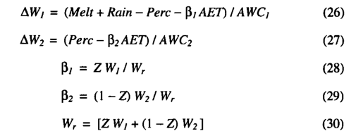
Soil hydrology. The soil is described by two layers at depths 0-500 mm and 500-1500 mm. Available water holding capacity (AWC, in millimetres) for each layer is defined as the difference between field capacity and wilting point for the relevant soil texture. Monthly rainfall totals are linearly interpolated to yield quasi-daily rainfall values. The soil moisture stores are updated each day using the daily percolation (Perc, in millimetres), quasi­daily rainfall (Rain, in millimetres), snowmelt (Melt, in millime-tres) and the calculated evapotranspiration rate (AET, in millimetres):

where Wj and W 2 are the soil water contents for the previous day (expressed as a fraction of the AWC in that layer); AWj and AW 2 are the daily changes in Wj and W 2 , respectively. AWCj and AWC2 are the available water holding capacities of the upper and lower soil layers, respectively. The parameters p ； and P 2 give the rates of extraction of transpired water from the upper and lower soil layers, respectively (such that py+p 2 =l). Zis a PFT specific parameter defining the fraction of the plants roots which are in the top soil layer. Wr is the average soil moisture in the rooting zone.

Percolation from the upper layer to the lower layer is calculated using an empirical equation adapted from Neilson [1995], The percolation formula is:

where Perc is the daily percolation (in millimetres) from the upper to the lower soil layer, K is an empirical parameter (in millimetres) dependent on soil texture, and Wj is the fractional wetness of the upper soil layer (as a fraction of the AWC). The equation is an empirical analog of Darcy's Law [Neilson, 1995] with conductiv­ity being represented as a power function of soil wetness (K gives the percolation rate when soil moisture in the upper soil layer is at field capacity). Percolation depends on soil texture through the value of K. Runoff occurs from the upper layer when the upper layer reaches field capacity and from the lower layer when the lower layer reaches field capacity.

Daily precipitation is defined as rain or snow depending on temperature being above or below -2°C. Snow melt is driven by temperature scaled by a melt coefficient:

where T_d is the quasi-daily temperature and 5m = 0.7 mm °C^-1d^-1.No snowmelt is allowed when the snowpack is depleted.

Soil moisture on day one is estimated by initializing the soil moisture stores at a value scaled to annual rainfall and then run­ning the water flux and phenology models for an initial spin-up year. Soil moisture values predicted for the last day of this spin-up year are then used for initializing a final run.

Values for the soil-texture dependent parameters are given in Table 3. The parameter K was calibrated so as to give magnitudes and ranges of percolation consistent with the four basic soil texture classes. AWC for each layer was calculated as the product of the volumetric water holding capacity (Hmax) and the depth of the soil layer. Values for  were calculated following the method de­scribed by Prentice et al. [1992]. The soil hydrology and evapotranspiration schemes have been extensively tested against highquality soil hydrological and micrometeorological data during a recent workshop on soil moisture simulation [Shao et ai, 1994],

Respiration costs. Whole plant respiration is calculated at a yearly time step as

where R_total  is the total annual plant respiration costs, R_leaf is an­nual leaf respiration, R_transport is annual maintenance respiration costs for transport tissues (e.g., stem and woody root sapwood), R_{fine_root} is fine root respiration, and R_growth is annual growthrespiration.

Leaf respiration costs are calculated at a monthly time step by the photosynthesis model and summed to obtain R_leaf.

Maintenance respiration for transport tissues is modeled as a function of the estimated total carbon content (Cs) of transport tissues. C 8 is estimated as a simple function of leaf area index (LAI) following the **pipe moder* theory of plant form [Shinozaki etal, 1964]:

where C_s is the total sapwood carbon content (kg C m'2), LAI is the leaf area index, and Cn is a parameter for the sapwood carbon content per unit LAI (kg C m"2). An average value for Cn was estimated by combining estimates of the proportion of biomass in sapwood [Ryan, 1989; Rogers and Hinckley, 1979] with estimates of average standing biomass from Olson et al. [1983] and Larcher [1983], resulting in the value of Cn being set equal to 1 kg C m'2.A modified Arrhenius relationship is used for the dependence of transport tissue maintenance respiration on temperature, following Lloyd and Taylor [1994]:

where m is the number of the month and Tc is the mean monthly temperature (in degrees celcius), Kr is the sapwood respiration rate(gC kg^-1C month^-1) at the reference temperature (T_ref) of 10°C, E_a=308.56 K, and T_a=-46.02°C. A mean value for Kr of 1.67 g C kg "1 C month_i was estimated from data presented in Table 2A of Sprugel et al. [1996].

Raich and Nadelhoffer [1989] presented data, from a wide range of forest ecosystems in different climate zones, that showed a strong correlation between total belowground carbon allocation(B_a) and total annual leaf litterfall carbon (L_f). They derived an equation for total annual below ground carbon allocation, B_a=130+ 1.92 L_f. However, the intercept was not significantly different from zero. We make the assumption that when averaged across all vegetation types, Ba will tend to zero as Lf tends to zero, implying that BJLf = 2. Furthermore, fine root construction and mainte­nance respiration are thought to account for about half of Ba [Sprugel et al., 1996; Ryan, 1991; Runyon et al.t 1994] leading to the simple approximation

where a=1. Leaf litterfall can be calculated from LAI, specific leaf area (SLA), and leaf longevity. Data presented by Reich et al. [1992] show that SLA decreases with leaf longevity in such a way as to keep litterfall approximately constant across the continuum from short-lived deciduous leaves to long-lived evergreen leaves, suggesting a simple relationship between litterfall and LAI:

where LAI is the leaf area index and Ln is the total annual leaf litterfall per unit leaf area. The value of Ln was estimated as 50 g Cm^-2 from relationships given by Reich et al. [1992]. Growth res­ piration (/?growth) is estimated as  20 % of the gross photosynthate remaining after all other respiration costs have been removed [Ryan, 1991].

Plant Functional Types

Just five woody and two grass plant functional types (PFTs) are used in the model. Differences in physiology, phenology and root­ing depth between the PFTs result in differences in their perfor­mance in the carbon and water flux model.

Rooting Depth. Grass roots are assumed to extract water al­most entirely from the upper soil. Woody plants extract water from both the upper and lower soil layers (Table 4). The rooting depth parameters follow Haxeltine et al. [1996].

Photosynthesis Rates for Evergreen Conifers. Evergreen needle-leaved conifers are assigned lower rates of photosynthesis (Table 4), based on the observation that photosynthetic rates decrease with increasing needle age  1982; Reich et al.t 1992]. Maximum photosynthetic rates for evergreen coni­fers typically decline at 30-50% per year [Chabot and Hicks, 1982]. However, older needles tend to occupy lower light envi­ronments in the interior of the canopy [Schulze et al., 1977], so the decrease in maximum photosynthetic rate with age at the needle level results in a much smaller decrease in whole-canopy photo­synthesis [Chabot and Hicksy 1982]. We assume, however, that this phenomenon is not solely due to needles adapting to increased shading and that it is partly due to specific characteristics of ever­ green conifer needles, possibly related to winter survival adaptations. Thus the implicit assumption is made that evergreen conifers have a mean needle age  >1 year, whereas deciduous trees have a mean leaf/needle age  ^1 year.

Minimum Conductances. A lower value of the minimum can­opy conductance is assigned to conifer plant types than to broad­ leaved plant types (Table 4) based on observations summarized by Kdrner [\994]. Similarly, the warm grass plant is assigned a high­er value of minimum stomatal conductance.

Phenology. Each PFT was assigned to be evergreen, summergreen, or raingreen (Table 4). For evergreen PFTs, leaf area is assumed constant through the year. For summergreen PFTs, leaf growth starts when the temperature rises above 5°C and takes a specified number of growing degree-days on a 5°C base (GDD, defined as GDD = ∑ (T_d-T_oo), where T_d is mean daily temperature, T_oo is the minimum temperature for growth, and summation is over the number of days in the year with T_d＞T_oo) to reach the maximum growing season leaf area (200 GDDs for summergreen woody PFTs, and 50 GDDs for the summergreen grass PFT). For raingreen PFTs a phenology algorithm was produced by calibrating soil moisture thresholds against observed raingreen phenologies: leaf area is reduced to zero whenever the soil moisture (lVr) in the rooting zone falls below 20% of the AWC in the rooting zone and is increased stepwise to the prescribed value when Wr rises above 30% of AWC in the rooting zone.

This simple phenology algorithm allows deciduous plant types to adopt an evergreen growth form under certain climates (i.e., summergreen trees growing in a climate with no monthly temper­ature below 5°C or raingreen trees growing in an environment with no dry period). In climates where this occurs, the deciduous plant type is allowed to be present but not dominant.

The cool grass plant type with its summergreen phenology is assigned if the temperature of the coldest month is below 5WC, otherwise the warm grass plant type with its evergreen phenology and slightly higher minimum canopy conductance is assigned.

Selection of C 4 Versus C 3 Grasses. Grasses may utilize either the  C₃  or  C₄  photosynthetic pathway, whereas woody plant types always use the  C₃  photosynthetic pathway (Table 4). C₄ grasses may have a lower canopy conductance and/or a higher photosyn­thesis rate than  C3  grasses. Both of these effects can give the  C₄ grass a competitive advantage. Furthermore, the benefits incurred through having a lower canopy conductance depend upon the moisture supply over the entire growing season. Thus both tem­perature and moisture stress will influence the relative competi­tiveness of  C₄ versus  C₃ grasses.

In the model, the choice of a  C4  or C 3 grass type is made on a monthly basis thus allowing seasonal changes in the dominance of C₄ or C₃ grasses. The model simulates the competitive balance between C₄ and C₃ grasses under conditions of moderate water stress, as found in most grassland ecosystems. Where water is limiting, the water use efficiency (defined as net photosynthesis/transpiration) gives a better measure of the realizable photo­synthesis rate than the non-water-stressed photosynthesis rate; and thus the water use efficiency more nearly defines competitive abil­ity than the non-water-stressed photosynthesis rate. Conceptually, the model selects the grass type which can achieve the highest monthly water use efficiency as dominant. C₄ grasses are selected when the monthly temperature is sufficient for C₄ grasses to have a higher rate of photosynthesis than C₃ grasses under the constraint of a normalized transpiration rate (defined by setting A<=0.4 for both plant types). For an ambient CO₂ concentration of 340 ^imol mol'1, the model predicts a transition in the dominant grass type from C₃ to C₄ grasses at a monthly mean temperature ( 7 ^ 4 ) of 15°C.

Ambient CO₂ concentration also influences the competitive balance between C4 and C₃ plants. As CO₂ concentration increas­

es, the photosynthesis rate of C₃ plants increases relative to C₄ plants; the temperature (T_C4) at which there is crossover from C₃ to C₄ grasses thus increases with CO₂  concentration. Furthermore, the photosynthesis model predicts a near linear increase in T_C4 with increasing CO₂ concentration. Using the photosynthesis model to calculate  7^4 at a range of ambient CO₂ concentrations, we developed the following regression equation for the calculation of  T_C4 at different CO₂ concentrations:

where ca is the ambient CO 2 mole fraction (μmol mol^-1).

Prediction of Equilibrium Leaf Area and NFP

Fundamental to BIOME3 is the method used to calculate leaf area as a function of moisture and carbon limitations. Haxeltine et al. [1996] reviewed several approaches that have been used for estimating large-scale patterns of sustainable leaf area as a func­tion of soilmoisture availability. They showed that the simulation of maximum sustainable leaf area in water-limited environments involves capturing the balance between two opposing effects. First, water-limited vegetation will tend to support as large a leaf area as water supply allows. Second, high transpiration rates due to excessive leaf area will ultimately reduce biomass production and impair plant vigor. The problem of estimating leaf area can therefore be regarded as an optimization problem in which the benefits of increasing leaf area in terms of light interception are traded off against the costs in terms of transpiration. Haxeltine et al. [1996] suggested that these benefits and costs may be expressed through NPP and that the optimization described above is concep­tually equivalent to maximizing NPP with respect to leaf area. The increasing costs of leaf respiration as leaf area increases are also included in the optimization of NPP.

However, the NPP obtained at a certain leaf area must also be sufficient to satisfy allocation requirements. This additional con­straint is important in environments where NPP and leaf area are limited by factors other than the water supply. In such environ­ments, such as high-latitude ecosystems, leaf area may instead be limited by an inability to satisfy whole-plant carbon allocation re­quirements at high leaf areas. We use the annual leaf litterfall Lf as an estimate of the absolute minimum allocation requirement. If at a certain leaf area NPP<%, the leaf area is considered unsupportable and is not allowed. Then, in the absence of water limitations, the equilibrium leaf area of the vegetation is the highest leaf area for which this minimum allocation requirement is still satisfied.

On the basis of this logic the model calculates an optimal NPP and leaf area for each PFT that may potentially be present in a certain grid square. This is done by calculating NPP at a compre­hensive range of leaf areas. The leaf area which gives the highest NPP, while still satisfying the minimum allocation constraint, is selected as being the optimal leaf area for that particular PFT in that grid square.

Simulation of the Dominant Plant Type

Selection of dominant PFTs is carried out using the NPP of one PFT relative to the NPP of another PFT as an index of the relative competitive ability of these two PFTs. This is done by first se­lecting a dominant woody PFT and then dealing with competition between the dominant woody PFT and grass PFT. The dominant woody PFT is selected from those potentially present in the grid square by selecting the woody PFT with the highest predicted NPP.

The competitive balance between woody plants and grasses in a savanna ecosystem is primarily determined by competition for available soil water [Walter, 1971; Walker and Noy-Meir, 1982; Knoop and Walker, 1985; Eagleson and Segarra, 1985; Neilson, 1995; Haxeltine et al„ 1996]. Important modifying factors are differences in physiology, fire disturbance, and competition for light [Daubenmire, 1978; Walter, 1979; Walker and Noy-Meir, 1982; Hopkins, 1992; Neilson, 1995]. The simulated NPP values capture the effects of competition for water resources and differ­ences in physiology but not light competition or fire disturbance.

In moist environments, trees will tend to form a dosed canopy which excludes grasses through light competition. Furthermore, fire frequency tends to be lower in moist environments than in dry environments, and frequent fires tend to favor the dominance of grasses. Through both of these mechanisms, moist environments tend to favor woody plants to the exclusion of a significant grass cover. Fire and light competition are not mechanistically modeled in BIOME3. Instead, these effects are empirically modeled by ex­cluding grasses if the annual average available soil moisture predicted for the dominant woody PFT is >75% (where 0% avail­able soil moisture is at the wilting point and  100 % is at field capacity) or if the annual rainfall is >2200 mm. If grasses are not excluded on the basis of this moisture rule, the PFT with the high­est NPP is predicted to be dominant. The competition algorithm is used to distinguish between environments in which woody plants are dominant (where woody NPP > grass NPP) versus environ­ments in which either a grassland or savanna is the dominant vegetation type (where grass NPP > woody NPP). In either case the modeled vegetation characteristics for the PFT with the highest NPP are assumed to be representative of the vegetation as a whole. In a earlier version of this model [Haxeltine et ai, 1996], compe­tition was handled by directly simulating the performance of different combinations of grass and woody plant types. The sim­plification made here is to simulate the competition between grasses and woody plants by comparing the performance of a grassand woody plant type growing separately. This simplification was found to give very similar results while saving dramatically on computational costs.

Mapping to Biomes

BIOME3 predicts the NPP, the LAI, the dominant PFT, and any secondary PFTs for each grid cell. This basic model output and a number of subsidiary variables are then used to assign a biome type according to the classification scheme shown in Table 5.