Quoted from: https://ccmc.gsfc.nasa.gov/models/models_at_glance.php 

Model Description
The GL model in its original form, describes the self similar expansion of a three-dimensional flux rope from the solar corona that offers a description of CMEs. The GL magnetic field takes the form of a closed magnetic flux rope which for our purpose is linearly superimposed on the background field of the AWSoM coronal and anchored (line tied) to the inner boundary of the model. The GL model also includes a density structure characterized by cold dense plasma located over the polarity inversion line surrounded by hot low-density plasma the fills the upper extremity of the flux rope. This density structure is embedded in the coronal model along with the magnetic field to produce a filament-cavity structure commonly observed to give rise to CMEs. Thus the GL model has the capability of reproducing both the magnetic and density structures of CMEs continuously from the low corona to Earth and beyond (e.g. Manchester et al. 2004a Manchester et al. 2014). With the GL flux rope inserted in the corona, the eruption occurs immediately from an initial state of force imbalance due to the magnetic pressure of the flux rope. Thus model eruption is entirely impulsive and lacks a gradual buildup or low acceleration of slow CMEs. However, the model quickly relaxes to realistic levels of CME deceleration after traveling to a distance of approximately 5 Rs from the solar surface.

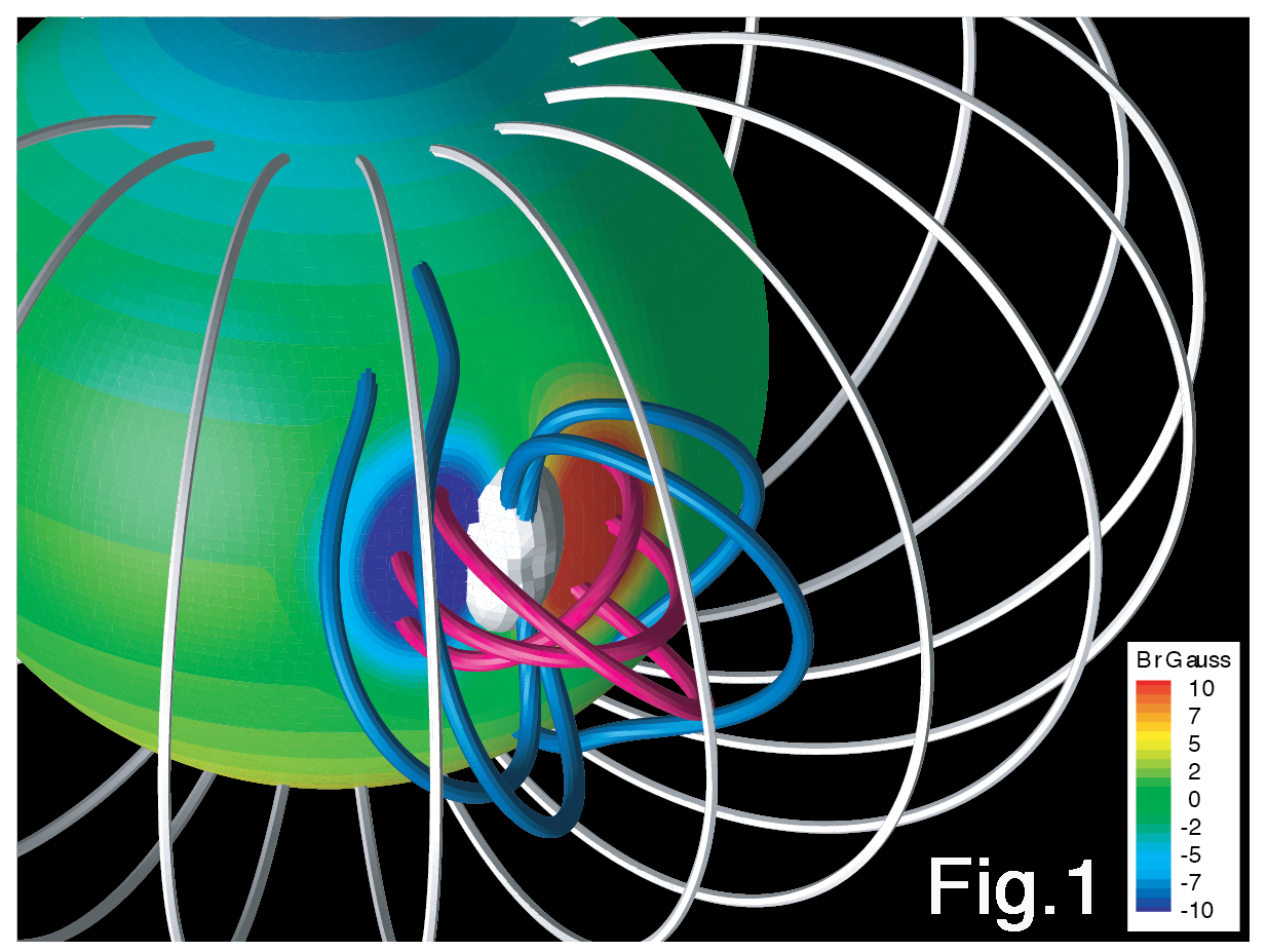
Fig 1: Isolated GL flux rope in dipole field. The radial magnetic field strength at the solar surface is given in color showing the footpoints of the flux rope in red/positive and blue/negative. Toroidal and poloidal flux are shown in red and blue respectively while dense filament material is shown as a white isosurface.

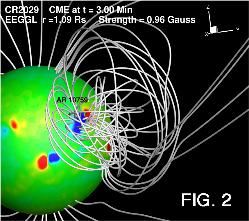
Fig 2: The GL flux rope embedded in the AWSoM coronal model for Carrington Rotation 2029. The color image of the solar surface provides the radial magnetic field strength while magnetic field lines are shown in gray. Here, the rope is clearly seen over the active region 10759, which produced a fast Earth-directed CME on 2005 May 13.

Model Input

GL Model Input:
The GL model is specified by a just a few parameters. First is the location and orientation of the flux rope on the solar surface. EEGGL allows the end-user specify the source region for the CME by identifying the originating active region as seen in a global synoptic magnetogram. The user clicks on the main negative and positive magnetic polarities of the active region for which EEGGL calculates the flux weighted centroid and provides its location (longitude and latitude in Carrington coordinates). EEGGL also performs a spline fit to the polarity inversion line and provides its orientation angle as measured relative to the solar equator. The location and orientation angle are provided as input parameters for the CME model so that GL flux rope is centered in the active region and the polarity inversion line of the rope coincides with that of the active region. Thus the filament material of the model will also be in the appropriate location.

The remaining parameters are the flux rope radius and field strength parameters. The radius is simply the radius of the sphere that contains the toroidal flux rope of the GL model. EEGGL scales the size of the flux rope to be proportional to the length of the polarity inversion line, and large enough to roughly fill the closed field region over the active region. The field strength is calculated by EEGGL to reproduce the CME speed in the low corona as provided by Stereo-CAT. This calculation is based on an empirical relationship between CME speed and the amount of reconnected magnetic flux in CME ejected flux ropes as measured in the associated flare ribbons.

The CME region should have refinement at level 6, extending +-40 degrees of the GL flux rope in longitude and +-20 degrees of the GL flux rope in latitude, and extend in radius is from 1.1 to 20.0. This refined grid region is specified by the AMRREGION type CMEbox as shown below. The IH grid show should also be refined, with the same angular extent as the SC grid, but extending from the IH inner boundary near 20 Rs to 1 AU, with a grid resolution of 0.5 Rs.

#AMRREGION
CMEbox
box_gen
1.1 RadiusMin (fixed)
-40.0 LongMin
-20.0 LatMin
20.0 RaduisMax (fixed)
40.0 LongMax
20.0 LatMax

Model Output
TBD

References and relevant publications

• Gibson, S. and Low B. C. A Time-Dependent Three-Dimensional Magnetohydrodynamic Model of The Coronal Mass Ejection, Astrophysical Journal, 493, 460-473, 1998.
• Manchester IV, W., Gombosi, T., Roussev, I., DeZeeuw, D.L., Sokolov, I., Powell, K., Toth, G., and Opher, M. Three-Dimensional MHD Simulation of a Flux Rope Driven CME, Journal of Geophysical Research, 109, A01102, doi:10.1029/2003JA010150, 2004.
• Manchester IV, W., Gombosi, T., Ridley, A., Roussev, I., DeZeeuw, D.L., Sokolov, I., Powell, K., and Toth, G., Modeling a Space Weather Event from the Sun to the Earth: CME Generation and Interplanetary Propagation, Journal of Geophysical Research, 109, A02107, doi10.1029/2002JA009672, 2004.
• Manchester IV, W. B., van der Holst, B., and Lavraud, B., Flux Rope Evolution in Interplanetary Coronal Mass Ejections: The 13 May 2005 Event, Plasma Phys. Control. Fusion, 56, 64006, 2014.

Relevant links

• SWMF website
• Eruptive Event Generator (Gibson and Low) - EEGGL
  • About EEGGL
  • Basic instructions on EEGGL use
• AWSoM_R + EEGGL

CCMC Contact(s)
Aleksandre Taktakishvili
301-286-4521

Developer Contact(s)
Igor Sokolov