The LPJ-DGVM has adopted many features from the BIOME family of models (Prentice et al., 1992; Haxeltine & Prentice, 1996a; Haxeltine et al., 1996; Kaplan, 2001). Bioclimatic limits as introduced in BIOME1, later used in BIOME3, have also been adopted in LPJ. Vegetation in a grid cell is described in terms of the fractional coverage of populations of different plant functional types (PFTs). Modellers define PFTs to account, in a very general way, for the variety of structure and function among plants (Smith et al., 1997). We define 10 PFTs, of which eight are woody (two tropical, three temperate, three boreal) and two herbaceous (Tables 1 and 2), following similar logic to that used in equilibrium biogeography models of the BIOME family (Prentice et al., 1992; Haxeltine & Prentice, 1996a; Haxeltine et al., 1996; Kaplan, 2001). In addition to the attributes controlling physiology and dynamics, each PFT is assigned biocli­ matic limits which determine whether it can survive and/or regenerate under the climatic conditions prevail­ing in a particular grid cell at a particular time in the simulation (Table 2) (Sitch, 2000; Venevsky, 2001). Bioclimatic limits follow the BIOME family except the continentality index for the boreal needle-leaved summergreen (Tw_c,min), which is derived by empirically fit­ting the distribution of Larix spp. to the modern climate(Venevsky, 2001).

Unlike previous models in the family, LPJ also includes explicit representation of vegetation structure, dynamics, competition between PFT populations, and soil biogeo­ chemistry. Figure 1 shows the model logic. The simulation in any grid cell is driven by input of monthly climatology, soil type and atmospheric C 〇 2 concentration, from which daily potential evapotranspiration and monthly soil temperatures are derived. The seasonal course of leaf phenology is then calculated for summergreen PFTs. Gross primary production (GPP) is calculated for each PFT population applying the coupled photosynthesis and water balance scheme of BIOME3. Maintenance and growth respiration are subtracted, and tissue turnover reduces individual plant biomass, with dead leaf and root tissue entering the litter pools. After subtracting a reproduction cost, the remaining photosynthate is allo­ cated to the C-compartments, satisfying four allometric relationships (see Section Average individual properties). Population densities are updated annually based on es­tablishment andmortality. Litter and soil organic matter(SOM) decomposition are driven by seasonal tempera­tures and soil moisture status.

Average individual properties  The fundamental entity simulated in LPJ is the average individual of a PFT. This concept provides a simple way for processes acting at the level of the plant individual to be scaled up to the ’population' over a grid-cell. In principle every higher plant species belongs to a PFT, whose physiology and dynamics are governed by a small set of key attributes. The current PFT classification is rather simple and capable of further development pending progress in PFT classification and characterization (Smith et al.,1997). The currently defined PFTs and their attributes are listed in Table 1. A small set of bioclimatic limits constrains PFT survival and regeneration (Table 2). The limits are applied to 20-year running means, not to annual or instantaneous values of the climate variables. This device allowed us to use limit values previously determined for biogeography models (e.g. Prentice et al.,1992; Haxeltine & Prentice, 1996a). Each PFT ’population' is characterized by a set of variables describing the state of the average individual, and by the population density(P). For woody PFTs (Table 1) the average individual is defined by its crown area (m2) and the sizes of four tissue pools (gC): leaf mass (Cleaf), sapwood mass (Csapwood), heartwood mass (Cheartwood), and fine root mass (Croot). Herbaceous PFTs are treated more simply by a ’big leaf' approximation; population density is arbitrarily set to 1, so that leaf mass and fine root mass represent grid cell area-averages (g Cm—2), while sapwood and heartwood mass are undefined.

Four scaling rules define individual physiognomy and constrain biomass allocation among the three living tissue pools (leaves, fine roots and sapwood) in woody plants:

1. The pipe model

where LA is the average individual leaf area (m²), SA(m²) is the sapwood cross sectional area and k_la:sa is aconstant (Table 3). This relationship is based on numer­ous studies indicating that each unit of leaf area must be supported by a corresponding area of transport tissue (Shinozaki et al.f 1964a,b; Kaufmann & Troendle, 1981;Waring et al.f 1982; Ryan, 1989; Robichaud & Methven, 1992; Berninger & Nikinmaa, 1994).

2. Functional balance

A second relationship relates investment in fine roots to investment in leaves and further requires plants in water-limited environments to allocate relatively more resources to fine root biomass. This results in an in­ creased maintenance respiration cost and a loss of poten­tial photosynthetic tissue as the cost of having to acquire water and nutrients (Larcher, 1983; Jackson et al., 1996). This relationship is expressed as:

where  oj is a value in the range 0-1 representing the current degree of water stress facing the average individ­ ual (see Section Water availability), while lrmax is the max­ imum leaf-to-root mass ratio (Table 3).

3. Stem mechanics

A standard allometry relates vegetation height to stem diameter (e.g. Huang et al., 1992).

where  k_allom2, k_allom3 are constants (Table 3).

4. Packing constraint

We use a relationship between crown area and stem diameter based on the inversion of Reinecke's rule(Zeide, 1993):

where k_allom1 and k_rp are constants and k_rp ≈1.6. Crown area is constrained not to exceed a constant, maximum CA_max (Table 3). Reinicke's rule relates tree density to stem diameter under self-thinning conditions, i.e., neigh­bourhood-scale survivorship. The inversion used here thus gives the expected relationship between individual crown area and stem diameter, assuming canopy closure but no overlap between crowns of adjacent individuals. Restriction of population density due to self-thinning is modelled in the mortality routine.

A combination of allometries 1-4 implies an increasing sapwood respiration cost with plant height, for a given leaf area. The relative contribution of sapwood respir­ation to the overall plant respiration increases with height, and is comparable to that of the other tissue respiration costs in tall individuals. Increasing respir­ation costs eventually restrict individual plant growth.

Other average individual properties

Other properties of the average individual can be de­rived from the state variables. The leaf area index of an individual is given by

where SLA is specific leaf area (m2gC_1). We employ an empirical relationship derived by Reich et al. (1997) relat­ing SLA to leaf longevity:

where aleaf is a PFT-specific value for leaf longevity in years (Table 1). This is an important relationship with respect to competition between PFTs because it helps to determine whether a deciduous or evergreen strategy is best suited to a given climate.

Leaf area index may be related to foliage projective cover (FPC) (Specht, 1970,1972,1981), defined as the area of ground covered by foliage directly above it, by the Lambert-Beer law (Monsi & Saeki, 1953):

Grid cell properties  The overall fractional coverage (FPC) of a PFT in a grid cell is obtained by multiplying average individual FPC with crown area and population density:

Consequently, the grid cell is treated as a mosaic divided into fractional coverages of PFTs and bare ground. However, it is assumed that the physical envir­onment of the plants is well mixed, i.e., the PFTs do not occupy discrete blocks, but compete locally for resources. Average individual carbon pools are similarly scaled to the grid cell by multiplying by population density.

Each PFT has an associated above- and below-ground litter pool (C _{l , ag}and C _{l , bg} , gCm^-2). Two soil pools, with ’intermediate' 卜 30years) and 'slow '( 〜1000 years) turn­ over times, respectively, are defined for the entire grid cell.

Annual vegetation and carbon dynamics  The current FPC  from Eqn. (8), used as a surrogate for FPAR, the daily leaf phenological status (i.e. fraction of full leaf cover) and climate data are used to calculate GPP for each PFT. This calculation is performed for the middle day of each month and daily values are derived by interpolation between the mid-month values. Maintenance respiration is calculated each simulation day based on the size of the living tissue pools, their assigned C:N ratios (cn) and climate data. Growth respiration, the cost of producing new tissues, is taken as a fraction of net primary pro­duction (NPP). Subtracting maintenance and growth res­piration from GPP gives NPP for each PFT. After subtracting an annual reproduction cost from NPP the remaining carbon is available for producing new tissue and is allocated to the living tissue pools of the PFT average individual in such a way as to satisfy the four scaling rules (Eqns 1-4). Tissue pools are also updated annually to account for tissue senescence/turnover (based on assigned turnover times) with carbon entering the litter (for leaves and fine roots) or (for sapwood) the nonliving heartwood pool.

The sum among PFTs of grid cell FPC is constrained to a maximum value of unity. If tissue growth in a par­ticular year leads to a grid cell FPC sum greater than unity, herbaceous PFT biomass is first reduced (repre­senting the competitive dominance of the taller-growing woody PFT's). If the grid cell FPC sum for woody vegetation exceeds an arbitrary limit of 0.95, woody PFT population is reduced, representing self-thinning. Additional mortality (reduction in population density) can result from depressed growth efficiency, heat stress, negative NPP and when a PFT's bioclimatic limits are exceeded.

The number of new individuals established annually is the product of the PFT-specific potential establishment rate and the fraction of the grid cell currently devoid of woody vegetation, i.e., areas sufficiently illuminated to allow sapling growth. Whether a particular PFT can establish depends also on available soil moisture and bioclimatic limits.

Phenology

Each woody PFT is assigned an evergreen, summergreen or raingreen phenology. Under water- or temperature-limited conditions herbaceous PFTs adopt a raingreen or summergreen phenology, respectively; otherwise, they are treated as evergreens.

Evergreen PFTs maintain constant leaf coverage over the year, and are assigned leaf longevities (^leaf) ^ lyear(see Table 1).

For summergreen PFTs, leaf-phenological status ⑷, updated daily, is defined as the current fraction of this year's maximum leaf coverage. Budburst occurs when daily temperature (Td) exceeds a minimum base tempera­ture (Tbase)- Leaf cover then increases in proportion to the accumulated heat sum (degree-days above TWse) until a PFT-specific limit for this heat sum (S gdd ) is reached (Table 1). Leaf senescence occurs once daily tem­peratures again fall below Tbase-

Maximum leaf coverage for raingreen PFTs is main­tained so long as the water stress factor,  oj (see below) remains above a threshold value of 0.35. Leaf senescence occurs if ω falls below 0.35.

Production

Water availability Soil hydrology is modelled following the semi-empirical approach of Haxeltine & Prentice (1996a), which was simplified, from the model developed by Neilson (1995). Two soil layers of fixed thickness (0.5 m upper and 1 m lower) are defined. The water con­tent of each layer is updated daily taking into account snowmelt, percolation, rainfall, evapotranspiration and runoff. Precipitation falls as rain or snow depending on whether the daily air temperature is above or below -2℃. Above this threshold the snow pack begins to melt at a maximum rate of

where T_d is the daily air temperature in ℃ and  k_melt is a constant (Table 3). Daily percolation from the upper to the lower soil layer is calculated using the empirical relationship of Neilson (1995),

where k_perc represents the soil texture dependent percola­tion rate (mm d^-1) at field capacity (Table 4) and W1 is the volumetric water content of the upper layer expressed as a fraction of its available water holding capacity. Surface runoff and drainage are calculated as the excess water above field capacity in the upper and lower soil layers, respectively. Plant functional types differ in their rooting strategy, woody PFTs having a smaller fraction of their roots in the upper soil layer compared with herbaceous plants. Competition between PFTs for water resources is therefore implicit in the water balance routine.

Daily evapotranspiration is calculated for each PFT as the minimum of a plant- and soil-limited supply function (E_supply) and the atmospheric demand (E_demand):

Esupply is the product of plant root-weighted soil moisture availability and a maximum transpiration rate, E_max(Table 3). E_demand is calculated following Monteith's(Monteith, 1995; Haxeltine & Prentice, 1996a) empirical relation between evaporation efficiency and surface con­ductance,

where Epot is the equilibrium evapotranspiration rate calculated from latitude, temperature and fractional sun­shine hours, using a standard method based on the Prescott equation and a similar approximation for long waveradiation(Prentice etal.,1993); gpot is the nonwater-stressed potential canopy conductance calculated by the photosynthesis routine (see below), and  and am are empirical parameters (Monteith, 1995; Table 3).

The water stress factor (w) is calculated for each PFT as

A daily value of w is used to update phenological status for raingreen PFTs (see Section Phenology), and an annual average value is used in calculating this year's leaf to fine root mass ratio for the allocation routine (Eqn. 2).

Photosynthesis  A brief overview of the photosynthesis model is presented here; full derivations are given by Haxeltine & Prentice (1996a,b) and Sitch et al. (2002, un­

published). The Farquhar photosynthesis model (Farquhar et al., 1980; Farquhar & von Caemmerer, 1982), as generalized for global modelling purposes by Collatz et al. (1991,1992), underlies the model. The 'strong optimality' hypothesis  (Dewar,  1996; Haxeltine & Prentice, 1996b; Prentice et al., 2000) is assumed to apply; the nitrogen content and Rubisco activity of leaves are assumed to vary both seasonally and with canopy position in such a way as to maximize net assimilation at the leaf level. The resulting model has the form of a 'light-use efficiency' model but the underlying theory makes it possible to predict the light-use efficiency from environmental variables.  Photosynthesis by  plants adopting the C3 vs. C4 biochemical pathways are mod­elled in slightly different ways. For C3 plants assimilation A_nd (gCm^-2day^-1) is given by

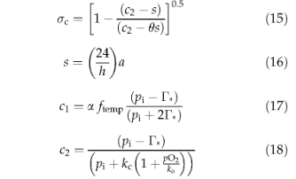
where i_d is the daily integral of absorbed photosynthetic­ally active radiation (PAR) calculated by a standard method (Haxeltine & Prentice, 1996a), including FPAR which is equal to FPC multiplied by phenology status; θ is the shape parameter which specifies the degree of colimitation by light and Rubisco activity (Haxeltine & Prentice,1996a,b); and the terms (Tc, s, a and & are given by:

where h is the day length in hours; a is a constant (leaf respiration as a fraction of Rubisco capacity; see Table 3); a is effective ecosystem-level quantum efficiency (Table 3); /temp is a PFT-specific temperature inhibition function limiting photosynthesis at low and high tem­peratures (Larcher, 1983; Sitch et al., 2002, unpublished); Γ_* is the CO₂ compensation point given by:

where pO₂ is the ambient partial pressure of  O₂(Pa); p_i is the intercellular partial pressure of CO₂(Pa) given by

where p_a  is the ambient partial pressure of CO₂ and λ is a parameter with a positive value ≤ 0.8. Parameters τ, k_o, k_c are kinetic parameters with a Q₁₀ dependence on temperature (Brooks & Farquhar, 1985; Collatz et al., 1991).

An appropriate simplification of the model (with dif­ferent values for a and a,λ≤0.8, and saturating p_i ) is applied for herbaceous plants with C₄ physiology (Haxeltine & Prentice, 1996a). The above equations de­scribe the biochemical dependence of total daily net as­similation on p_i and environmental variables.

The daytime assimilation rate A_dt is also related to p_i through the CO₂ diffusion gradient between the atmos­ phere and intercellular air spaces:

where g min  is a PFT-specific minimum canopy conduct­ance (scaled by FPC) and c_a is the ambient mole fraction of CO₂ (P_a = P*c_a  where p is atmospheric pressure). A_dt is obtained from And by addition of nighttime respiration.

Under nonwater-stressed conditions maximum values of λ(0.8 for C₃ plants; 0.4 for C₄ plants) are assumed; and is calculated from Eqn. (14) and g_c is derived from Eq.(21). The value for canopy conductance thus obtained is the potential canopy conductance, g_pot, required to derive demand-limited AET in Eqn. (12). If  oj < 1 (supply limitation of transpiration), Eqns (12), (14) and (21) are solved simultaneously to yield values of X and  consist­ent with the transpiration rate. Annual GPP is obtained by adding daytime respiration to A_dt and summing over the year.

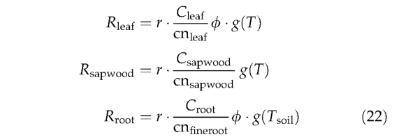
Autotrophic respiration Maintenance respiration is calcu­lated daily based on tissue-specific C:N ratios (cn), tem­perature (either air, T, or soil temperatures, T_soil (see Appendix Section), for above and below ground tissues, respectively), tissue biomass and phenology following the approach of Ryan (1991) and Sprugel et a/. (1995):

where

Equation (23) is a modified Arrhenius equation (Lloyd & Taylor,1994), where T is the temperature (°C). The use of such a relationship in preference to a fixed Q₁₀ is justified by evidence for a consistent decline in the apparent Q₁₀ of autotrophic respiration with temperature (Tjoelker et al.,1999). The PFT-specific parameter r is the respiration rate(gCgN-1day-1) on a 10 °C base. Chosen values of r crudely account for the observation that plants from warmer environments typically have much lower respir­ation rates at any given temperature than plants from cooler environments (Fukai & Silsburg, 1977; Lechowicz et al., 1980; Amthor, 1989; Ryan, 1991). Daily tissue main­tenance respiration rates are summed over tissues and days to give the annual maintenance respiration for the average individual of each PFT. Multiplying by the population density gives the PFTs total maintenance respiration over the grid cell:

After maintenance respiration is subtracted from GPP, 25% of the remainder is taken as growth respiration, the cost of producing new tissues, leaving the annual net primary productivity (gCm^-2yr^-1) (Ryan, 1991) as

Average individual growth

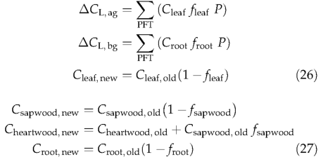
Tissue turnover Each living tissue is assigned a PFT-specific tissue turnover rate (Table 1) (Schoettle &Fahey, 1994), which is transferred either into litter (leaf and fine root), or from living sapwood to heartwood. Thus,

where C_L,ag and C_L,bg are thisyear's updated above-and below-ground litter, respectively.

Reproduction Reproduction costs - carbohydrate allo­cated to produce reproductive organs and propagules-range between 5% and 20% of NPP (Harper, 1977; Larcher, 1983). As a simple approximation, a fixed 10% fraction of annual NPP is deducted to account for allocation to reproduction. Only a minute part of this carbon enters the next generation, so in order to maintain a closed carbon cycle all of the reproductive allocation is assumed to enter the above-ground litter pool.

Allocation Once reproduction costs have been ac­ counted for, the remaining fraction of annual NPP, the biomass increment (ΔC), is allocated to the tissue pools in such a way as to satisfy the four scaling rules (Eqns 1-4), governing plant physiognomy. Thus,

where ΔC_leaf, ΔC_sapwood and ΔC_root represent thebiomass allocation to the respective pools. Equations (1-4) and (28) are combined and the individual allocation terms derived using standard numerical methods. In years of stress, the biomass increment may not allow sufficient allocation to the leaves to fully utilize the current sapwood (given the constraint implied by Eqn. 1). This year's production is then allocated to leaves and roots only, and the excess sapwood mass transferred to the nonliving heartwood pool. In a year with severe drought there may be insufficient biomass increment to maintain both current sapwood mass and leaf mass. In this case all of the biomass increment is allocated to fine roots and excess sapwood and leaf mass transferred to the heart-wood and above-ground litter pools, respectively.

For herbaceous plants, which lack wood, the biomass increment is distributed among leaves and fine roots according to Eqn. (2). Relocation of carbon is allowed from the fine roots to leaves, i.e., we assume the existence of below-ground carbon reserves, which can be mobilized in times of stress.

Vegetation structure (in terms of crown area and FPC) is updated after allocation of the biomass increment, in accordance with Eqns (1-4), (7) and (8).

Mortality

Mortality is imposed as a reduction in population density at the end of each simulation year. Mortality may occur as a result of light competition (mort shade ), low growth efficiency (mort g m ff ), a negative annual carbon balance (mort N pp ), heat stress (mort heat ), or when PFT bioclimatic limits are exceeded for an extended period (mort lim ). The overall mortality rate for a popula­tion is the sum of the rates for individual mortality components (maximum 1), i.e.,

The living biomass and heartwood of killed individuals is transferred to the above- and below-ground litter pools, i.e.,

Competition for light among neighbouring individuals occurs whenever increased biomass results in a grid cell FPC of more than 1, when summed across all PFTs, or more than 0.95, when summed across woody PFTs. Mortality is imposed such that summed woody FPC is reduced to 0.95, and/or total grid cell FPC is reduced to 1. Herbaceous plants are assumed to be inferior to woody plants in competition for light, and can occupy, at most, that proportion of the gridcell(1-FPC woody )not occupied by woody plants. Shading mortality is partitioned among woody PFTs in proportion to the FPC increment resulting from their biomass increment for this year. The same rule is applied for herbaceous plants. Background mortality is calculated from this year's growth efficiency (Waring, 1983; Waring & Schlesinger, 1985), the ratio of this year's net biomass increment to leaf area:

Following Prentice et al. (1993), the mortality rate is inversely related to growth efficiency:

where  K_mort1 represents the asymptotic maximum mortality rate, and K_mort2 is a parameter governing the slope of the relationship between mortality and growth efficiency (see Table 3). All individuals in a PFT population are killed if NPP becomes negative in any year:

During prolonged periods with high temperatures, some plants, especially those found in temperate and boreal ecosystems, can become stressed and suffer tissue damage. Heat stress could lead to forest dieback, as has been shown under climate warming scenarios (Joos et al., 2001). The formulation of heat damage mortality is based on the annual accumulated degree-day sum above a PFT-specific temperature base, Tmort^min (Table 1), with mor­tality increasing linearly and reaching unity (complete mortality) at or above 300 degree-days above the thresh­ old value:

If 20-year mean values of bioclimatic variables fall outside a PFTs limits for survival (Table 2), its entire population is killed (mort_lim=1).

Disturbance regime  Fire is the most important natural disturbance at a global scale, and is the only form of disturbance explicitly represented in LPJ. A full descrip­tion of the fire module is given by Thonicke et al. (2001).

Several simplifying assumptions are made. First, fire occurrence is taken to be dependent only upon fuel load (i.e. the amount of dry combustible material, C_L,ag ) and litter moisture. Fire spread is not possible below a min­imum fuel load, fuel min  (Table 3). Ignition sources are assumed to be available whenever fire is possible. Second, fire effects are assumed to be determined onlyby the length of the fire season and PFT specific 'resist­ances' (r_fire , Table 1).

A threshold value of fuel moisture content is defined as the value above which a fire would not spread. An expo­nential function is used to approximate the probability of the occurrence of at least one fire in a day:

where W_l,d is the daily moisture status in the upper soil layer, used here as a surrogate for litter moisture, and me is a PFT weighted threshold value (Table 3). The length of the fire season (in years) is taken as:

A constant, nonlinear relationship between length of fire season and annual area burnt is assumed.

The fraction of individuals killed within the burnt areas depends on the prescribed PFT fire resistance. Tropical raingreen and temperate broadleaved evergreen woody PFTs are relatively resistant to fire, reflecting widespread adaptations to fire among plants of dry subtropical and tropical environments. The other woody PFTs have lower resistance (Table 1). Herbaceous plants are assumed to complete their life cycle ahead of the fire season and are therefore unaffected by fire disturb­ance in the model.

The living biomass and heartwood of individuals killed by fire are assumed to be fully consumed, and released to the atmosphere as CO₂. Above-ground litter in the burnt fraction of a grid cell is likewise fully con­sumed and released as CO₂.

Establishment

Each year, new woody PFT individuals and herbace­ous PFTs are established, available space permitting. Woody PFTs are subject to a maximum establishment rate of 0.24 saplings m-2 (Prentice et al., 1993). Woody PFT saplings can establish in the proportion of the grid cell not currently occupied by woody PFTs, representing the illuminated understorey, or open ground; shading reduces establishment as summed woody FPC appro­aches its limit of 1. Woody PFTs within their bioclimatic limits for establishment have the same establishment rate given by:

where n_est,woody and FPC_woody are the number and summed FPC of woody PFTs within their bioclimatic limits for establishment (Table 2). The establishment rate increments population density:

while tissue biomass for the PFT average individual is modified to account for the addition of saplings (of pre­scribed biomass) to the PFT population; for each tissue(leaf, sapwood, heartwood, fine root):

Saplings are assumed to have an initial individual LAI of 1.5, from which initial biomass in each tissue is derived (by Eqns 1-4). Herbaceous PFTs can establish in nonve­getated area (not yet occupied by any PFT). The establish­ ment rate for each herbaceous PFT is given by:

where FPC_total  is the summed FPC of all PFTs (woodyand herbaceous); n_est,herb  is the number of herbaceous PFTs within their bioclimatic limits for establishment. The herbaceous establishment rate modifies leaf and root biomass:

where C_leaf,est and C_root,est are prescribed incremental leaf and fine root biomass values based on an LAI of 0.001.

Establishment of both woody and herbaceous PFTs is inhibited under extreme heat or water stress. A minimum annual precipitation limit (prec_min) of 100 mm is set, below which seedlings will not germinate and so no establishment will occur. Development of seedlings and saplings is not explicitly modelled through the course of the year. The additional uptake of carbon associated with sapling establishment is therefore simply added to the annual NPP. A major simplification arising from the average-individual approach is that only one age-height class for each woody PFT is explicitly defined for a grid cell at any particular time. By updating the status of the PFT average individual, sapling properties are merged with the extant average individual properties, effectively surpassing life cycle stages, which might significantly influence the dynamics of real vegetation. This represents a major simplification in the treatment of population dynamics in the model. However, subdivision of PFTs into age-height classes is technically possible within the design of LPJ and would be important, e.g., for modelling the effects of forest management.

Soil and litter biogeochemistry

Each PFT has an associated above- and below-ground litter pool. As litter decomposes a fraction, representing the highly labile fraction, is respired as CO2 directly into the atmosphere. The remainder is divided between the intermediate and slow SOM pools (Foley, 1995). The litter pool is assigned a decomposition rate at 10 °C of 0.35yr^-1 while the intermediate and slow SOM pools are assigned decomposition rates at 10 °C of 0.03 and 0.001yr^-1. These rates correspond to turnover times (τ₁₀) of 2.86,33.3,1000years, respectively (Meentemeyer, 1978; Foley, 1995).

Decomposition is soil temperature- and moisture-dependent. Temperature dependence follows the modi­fied Arrhenius relationship (Lloyd & Taylor, 1994) also used for modelling maintenance respiration in LPJ(Eqn. 23). Above-ground litter decomposition is made dependent on air temperature, whereas below-ground litter and SOM decomposition are related to soil tempera­ture. An empirical soil moisture relationship from Foley (1995) is adopted:

where W_i is the average moisture status in the upper soil layer in a given month. Monthly decomposition rates as a function of monthly temperature and moisture status are given by:

Decomposition follows first-order kinetics (Olson, 1963):

where C is the pool size, t is time and k the monthly decomposition rate. Integrating with respect to time t,

gives C, the pool size at any time t, with C₀ representing its initial size. The amount of carbon decomposed in one month is,

Following Foley (1995), 70% of the decomposed litter goes directly into the atmosphere as C 〇 2  (f_air), the remaining 30% entering the soil pools, with 98.5% (f_inter) and 1.5% 〇 (f_slow ) of theremainder entering the intermediate and slow soil pools, respectively. Summation of the monthly litter and soil decomposition terms gives total monthly heterotrophic respiration, R_h :

where Φ_utter,  Φ_inter and Φ_slow are carbon emissions from the litter pools, the intermediate and slow soil pools, respectively.

Input data

Monthly fields of mean temperature, precipitation and cloud cover were taken from the CRU05 (1901-1998) monthly climate data on a 0.5° x 0.5° global grid, pro­vided by the Climate Research Unit (CRU), University of East Anglia (New et al., 1999a,b, unpublished). Cloud cover data for 1997 and 1998, not so far compiled by CRU, were taken as the average over the previous 30 years. Monthly data were interpolated to provide 'quasi-daily' time series of climate. A data set of historical global atmospheric C 〇 2 concentrations extending from 1901 to 1995 was obtained courtesy of the Carbon Cycle Model Linkage Project (Kicklighter et al., 1999; McGuire et al.,2001). These data were derived from a combination of ice-core measurements (Etheridge et al., 1996) and atmos­pheric observations (Keeling et al., 1995). The dataset was extended to 1998 using the same procedure. Soil texture data were as in BIOME3 (Haxeltine & Prentice, 1996a), based on the FAO soil data set (Zobler, 1986; FAO, 1991).

From remote sensing (Advanced Very High Resolution Radiometer, AVHRR), Defries et al. (2000) generated a global map at 1 km spatial resolution of percentage tree cover, and maps partitioning the woody vegetation according to phenology (evergreen vs. deciduous) and leaf morphology (broadleaf vs. needleleaf) [http://glcf.umiacs.umd.edu]. These data were aggregated to a 0.5° x 0.5° grid for comparison with LPJ simulation results. Observations of atmospheric CO2 concentrations from a network of 27 monitoring stations were obtained from a programme of the National Oceanographic and Atmospheric Administration (NOAA) (GLOBALVIEW-CO2, 1999). The monthly station records were post-processed to extract the detrended, average monthly observations between 1983 and 1992 (Heimann et al.,1998). This same procedure was applied to model out­puts before the net monthly fluxes were passed to the atmospheric tracer transport model, TM2. Monthly fluxes of CO2 between the atmosphere and the ocean surface were obtained from a standard run of the Hamburg. Model of the Ocean Carbon Cycle (HAMOCC3, see Maier-Reimer, 1993) including a NPZD-type marine bio­sphere model (Kurz, 1993; Six & Maier-Reimer, 1996). Monthly CO2 emissions fields from fossil-fuel burningand cement manufacture were computed based on a global 1° x 1° map compiled by Marland et al. (1989),assuming constant emissions throughout the year(Heimann et al., 1998). Reduced-form 'station matrices'(see Kaminski et al., 1999a,b) were derived from the TM2 atmospheric tracer transport model (Heimann et al., 1989)using wind fields based on the 12-h analyses of the European Centre for Medium-Range Weather Forecasts for the year 1987. A global 1° x 1° data set of annual runoff was used (Cogley, 1991). Measurements of me­teorological data (temperature, precipitation and net in­ coming solar radiation), and fluxes of net ecosystem exchange, NEE, for six EUROFLUX sites were obtained courtesy of the EUROFLUX monitoring network [http://www.unitus.it/dipartimenti/disafri/progetti/eflux/euro.html]. Data for the soil moisture balance evaluation were provided by the Global Soil Moisture Data Bank [http://metosrv2.umd.edu/~alan/soil_moisture/ruswet. forcing.6sta.readme.html] (Robock et al.f 1995) and Goutorbe et al. (1989); Goutorbe & Tarrieu (1991); Cammeraat & Prinsen (1995); Cammeraat (1996) and Menzel (1997).

Modelling protocol

A typical simulation with LPJ starts from 'bare ground' (no plant biomass present) and 'spins up' for 1000 model years until approximate equilibrium is reached with re­spect to carbon pools and vegetation cover. It is appro­priate to drive the model with an approximately constant climate during the spin up phase; however, since fires in many regions occur only in drier years, repeating a single year's climate or even using a long-term climatic average, can lead to anomalous results. The spin-up therefore requires the use of an interannually varying climate, with annual-average temperatures, precipitation and cloudiness fluctuation about constant long-term means. In order to enhance computational efficiency, the size of the slow SOM pool is solved analytically after 400years. The spin-up is continued for a further 600 years to ensure closeness to equilibrium in the slower carbon pools. The model can then be driven with a transient climate.

In a standard simulation LPJ is run in the transient phase using the CRU data for 1901-1998. For the com­ parison against the EUROFLUX site climate data, the available monthly site data were first regressed against the corresponding CRU data, for the nearest grid cell, and then historical 1901-1998 site climatologies were con­structed. For seasonal soil moisture-balance analysis, the site climate data were used directly. 

To simulate seasonal cycles of atmospheric CO2 at the regional scale, monthly net carbon exchanges for each 0.5° x 0.5° grid cell over the globe were calculated from LPJ-predicted heterotrophic respiration, biomass burntand NPP, i.e.,

Detrended averages of NEE for 1982-1993 were derived as in Heimann et al. (1998) and used as input to an atmospheric transport model (Heimann et al., 1989), whose outputs were 'sampled' at the locations of the measuring stations.