Radial Basis Functions

Uses one of five basis functions to process each measured sample value, thus creating an exact interpolation surface

Interpolation

Contributor(s)

Initial contribute: 2019-05-09

Authorship

:  
View
Is authorship not correct? Feed back

Classification(s)

Method-focused categoriesData-perspectiveGeoinformation analysis

Detailed Description

English {{currentDetailLanguage}} English

Summary

Uses one of five basis functions to process each measured sample value, thus creating an exact interpolation surface.

Usage

  • The smooth search neighborhood is only available for the Inverse multiquadric function.

  • For all methods except the Inverse multiquadric function, the higher the parameter value, the smoother the surface. The opposite is true for the Inverse multiquadric function.

Syntax

RadialBasisFunctions_ga (in_features, z_field, {out_ga_layer}, {out_raster}, {cell_size}, {search_neighborhood}, {radial_basis_functions}, {small_scale_parameter})
Parameter Explanation Data Type
in_features

The input point features containing the z-values to be interpolated.

Feature Layer
z_field

Field that holds a height or magnitude value for each point. This can be a numeric field or the Shape field if the input features contain z-values or m-values.

Field
out_ga_layer
(Optional)

The geostatistical layer produced. This layer is required output only if no output raster is requested.

Geostatistical Layer
out_raster
(Optional)

The output raster. This raster is required output only if no output geostatistical layer is requested.

Raster Dataset
cell_size
(Optional)

The cell size at which the output raster will be created.

This value can be explicitly set under Raster Analysis from the Environment Settings. If not set, it is the shorter of the width or the height of the extent of the input point features, in the input spatial reference, divided by 250.

Analysis Cell Size
search_neighborhood
(Optional)

Defines which surrounding points will be used to control the output. Standard is the default.

This is a Search Neighborhood class SearchNeighborhoodStandard ,SearchNeighborhoodSmooth, SearchNeighborhoodStandardCircular, and SearchNeighborhoodSmoothCircular.

Standard

  • Major semiaxis—The major semiaxis value of the searching neighborhood.
  • Minor semiaxis—The minor semiaxis value of the searching neighborhood.
  • Angle—The angle of rotation for the axis (circle) or semimajor axis (ellipse) of the moving window.
  • Maximum neighbors—The maximum number of neighbors that will be used to estimate the value at the unknown location.
  • Minimum neighbors—The minimum number of neighbors that will be used to estimate the value at the unknown location.
  • Sector type—The geometry of the neighborhood.
    • One sector—Single ellipse.
    • Four sectors—Ellipse divided into four sectors.
    • Four sectors shifted—Ellipse divided into four sectors and shifted 45 degrees.
    • Eight sectors—Ellipse divided into eight sectors.

Smooth

  • Major semiaxis—The major semiaxis value of the searching neighborhood.
  • Minor semiaxis—The minor semiaxis value of the searching neighborhood.
  • Angle—The angle of rotation for the axis (circle) or semimajor axis (ellipse) of the moving window.
  • Smoothing factor—The Smooth Interpolation option creates an outer ellipse and an inner ellipse at a distance equal to the Major Semiaxis multiplied by the Smoothing factor. The points that fall outside the smallest ellipse but inside the largest ellipse are weighted using a sigmoidal function with a value between zero and one.

StandardCircular

  • Radius—The length of the radius of the search circle.
  • Angle—The angle of rotation for the axis (circle) or semimajor axis (ellipse) of the moving window.
  • Maximum neighbors—The maximum number of neighbors that will be used to estimate the value at the unknown location.
  • Minimum neighbors—The minimum number of neighbors that will be used to estimate the value at the unknown location.
  • Sector type—The geometry of the neighborhood.
    • One sector—Single ellipse.
    • Four sectors—Ellipse divided into four sectors.
    • Four sectors shifted—Ellipse divided into four sectors and shifted 45 degrees.
    • Eight sectors—Ellipse divided into eight sectors.

SmoothCircular

  • Radius—The length of the radius of the search circle.
  • Smoothing factor—The Smooth Interpolation option creates an outer ellipse and an inner ellipse at a distance equal to the Major Semiaxis multiplied by the Smoothing factor. The points that fall outside the smallest ellipse but inside the largest ellipse are weighted using a sigmoidal function with a value between zero and one.
Geostatistical Search Neighborhood
radial_basis_functions
(Optional)

Available Radial basis functions.

  • THIN_PLATE_SPLINE —Thin-plate spline
  • SPLINE_WITH_TENSION — Spline with tension
  • COMPLETELY_REGULARIZED_SPLINE — Completely regularized spline
  • MULTIQUADRIC_FUNCTION — Multiquadric function
  • INVERSE_MULTIQUADRIC_ FUNCTION —Inverse multiquadric function
String
small_scale_parameter
(Optional)

Used to calculate the weights assigned to the points located in the moving window. Each of the radial basis functions has a parameter that controls the degree of small-scale variation of the surface. The (optimal) parameter is determined by finding the value that minimizes the root mean square prediction error (RMSPE).

Double

Code Sample

RadialBasisFunctions example 1 (Python window)

Interpolate point features onto a rectangular raster.

import arcpy
arcpy.env.workspace = "C:/gapyexamples/data"
arcpy.RadialBasisFunctions_ga(
    "ca_ozone_pts", "OZONE", "outRBF", "C:/gapyexamples/output/rbfout", "2000", 
    arcpy.SearchNeighborhoodStandard(300000, 300000, 0, 15, 10, "ONE_SECTOR"),
    "THIN_PLATE_SPLINE", "")
RadialBasisFunctions example 2 (stand-alone script)

Interpolate point features onto a rectangular raster.

# Name: RadialBasisFunctions_Example_02.py
# Description: RBF methods are a series of exact interpolation techniques;
#              that is, the surface must go through each measured sample value.
# Requirements: Geostatistical Analyst Extension

# Import system modules
import arcpy

# Set environment settings
arcpy.env.workspace = "C:/gapyexamples/data"

# Set local variables
inPointFeatures = "ca_ozone_pts.shp"
zField = "OZONE"
outLayer = "outRBF"
outRaster = "C:/gapyexamples/output/rbfout"
cellSize = 2000.0
rbf = "THIN_PLATE_SPLINE"
smallscaleParam = ""

# Set variables for search neighborhood
majSemiaxis = 300000
minSemiaxis = 300000
angle = 0
maxNeighbors = 15
minNeighbors = 10
sectorType = "ONE_SECTOR"
searchNeighbourhood = arcpy.SearchNeighborhoodStandard(majSemiaxis, minSemiaxis, 
                                                       angle, maxNeighbors, 
                                                       minNeighbors, sectorType)

# Check out the ArcGIS Geostatistical Analyst extension license
arcpy.CheckOutExtension("GeoStats")

# Execute RadialBasisFunctions
arcpy.RadialBasisFunctions_ga(inPointFeatures, zField, outLayer, outRaster, 
                              cellSize, searchNeighbourhood, rbf, smallscaleParam)


Licensing Information

ArcGIS for Desktop Basic: Requires Geostatistical Analyst
ArcGIS for Desktop Standard: Requires Geostatistical Analyst
ArcGIS for Desktop Advanced: Requires Geostatistical Analyst


How radial basis functions work

RBF methods are a series of exact interpolation techniques; that is, the surface must pass through each measured sample value. There are five different basis functions:

  • Thin-plate spline
  • Spline with tension
  • Completely regularized spline
  • Multiquadric function
  • Inverse multiquadric function

Each basis function has a different shape and results in a different interpolation surface. RBF methods are a special case of splines.

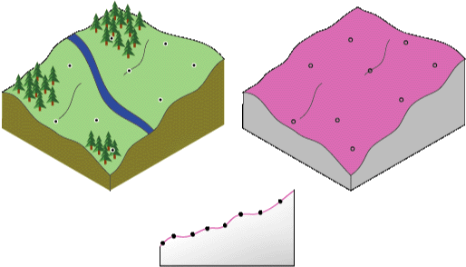
RBFs are conceptually similar to fitting a rubber membrane through the measured sample values while minimizing the total curvature of the surface. The basis function you select determines how the rubber membrane will fit between the values. The diagram below illustrates conceptually how an RBF surface fits through a series of elevation sample values. Notice in the cross section that the surface passes through the data values.

Radial Basis Functions

Being exact interpolators, the RBF methods differ from the global and local polynomial interpolators, which are both inexact interpolators that do not require the surface to pass through the measured points. When comparing an RBF to IDW (which is also an exact interpolator), IDW will never predict values above the maximum measured value or below the minimum measured value as you can see in the cross section of a transect of sample data below.

Inverse Distance Weighted profile

However, the RBFs can predict values above the maximum and below the minimum measured values as in the cross section below.

RBF cross section

Optimal parameters are determined using cross validation in a similar manner as explained for IDW and local polynomial interpolation.

    When to use radial basis functions

RBFs are used to produce smooth surfaces from a large number of data points. The functions produce good results for gently varying surfaces such as elevation.

However, the techniques are inappropriate when large changes in the surface values occur within short distances and/or when you suspect the sample data is prone to measurement error or uncertainty.

    The concepts behind radial basis functions

In Geostatistical Analyst, RBFs are formed over each data location. An RBF is a function that changes with distance from a location.

RBF concept diagram


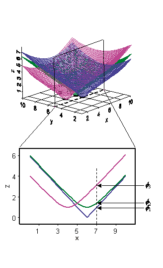
For example, suppose the radial basis function is simply the distance from each location, so it forms an inverted cone over each location. If you take a cross section of the x,z plane for y = 5, you will see a slice of each radial basis function. Now, suppose you want to predict a value at y = 5 and x = 7. The value of each radial basis function at the prediction location can be taken from the figure above, given by the values Φ1, Φ2 , and Φ3, which simply depend on the distance from each data location. The predictor is formed by taking the weighted average w1Φ1 + w2Φ2 + w3Φ3 + …

Now the question is how to determine the weights? So far, you have not used the data values at all. The weights w1, w2, w3, and so on, are found by requiring that, when the prediction is moved to a location with a measured value, the data value is predicted exactly. This forms N equations with N unknowns and can be solved uniquely. Thus, the surface passes through the data values, making predictions exact.

The radial basis function in this example is a special case of the multiquadric RBF. Geostatistical Analyst also allows you to use other RBFs such as completely regularized splines, thin-plate splines, splines with tension, and inverse multiquadric. Sometimes, the difference between these is not great, but you may have reason to choose one or you can try several and use cross-validation to select one. Each of the RBFs has a parameter that controls the "smoothness" of the surface.

RBF menu

For all methods except inverse multiquadric, the higher the parameter value, the smoother the map; the opposite is true for inverse multiquadric.

模型元数据

{{htmlJSON.HowtoCite}}

ESRI (2019). Radial Basis Functions, Model Item, OpenGMS, https://geomodeling.njnu.edu.cn/modelItem/2c155642-6e5c-43ca-a41a-9a51c18a80aa
{{htmlJSON.Copy}}

Contributor(s)

Initial contribute : 2019-05-09

{{htmlJSON.CoContributor}}

Authorship

:  
View
Is authorship not correct? Feed back

QR Code

×

{{curRelation.overview}}
{{curRelation.author.join('; ')}}
{{curRelation.journal}}


{{htmlJSON.RelatedItems}}

{{htmlJSON.LinkResourceFromRepositoryOrCreate}}{{htmlJSON.create}}.

Drop the file here, orclick to upload.
Select From My Space
+ add

{{htmlJSON.authorshipSubmitted}}

Cancel Submit
{{htmlJSON.Cancel}} {{htmlJSON.Submit}}
{{htmlJSON.Localizations}} + {{htmlJSON.Add}}
{{ item.label }} {{ item.value }}
{{htmlJSON.ModelName}}:
{{htmlJSON.Cancel}} {{htmlJSON.Submit}}
名称 别名 {{tag}} +
系列名 版本号 目的 修改内容 创建/修改日期 作者
摘要 详细描述
{{tag}} + 添加关键字
* 时间参考系
* 空间参考系类型 * 空间参考系名称

起始日期 终止日期 进展 开发者
* 是否开源 * 访问方式 * 使用方式 开源协议 * 传输方式 * 获取地址 * 发布日期 * 发布者


编号 目的 修改内容 创建/修改日期 作者


时间分辨率 时间尺度 时间步长 时间范围 空间维度 格网类型 空间分辨率 空间尺度 空间范围
{{tag}} +
* 类型
图例


* 名称 * 描述
示例描述 * 名称 * 类型 * 值/链接 上传


{{htmlJSON.Cancel}} {{htmlJSON.Submit}}
Title Author Date Journal Volume(Issue) Pages Links Doi Operation
{{htmlJSON.Cancel}} {{htmlJSON.Submit}}
{{htmlJSON.Add}} {{htmlJSON.Cancel}}

{{articleUploading.title}}

Authors:  {{articleUploading.authors[0]}}, {{articleUploading.authors[1]}}, {{articleUploading.authors[2]}}, et al.

Journal:   {{articleUploading.journal}}

Date:   {{articleUploading.date}}

Page range:   {{articleUploading.pageRange}}

Link:   {{articleUploading.link}}

DOI:   {{articleUploading.doi}}

Yes, this is it Cancel

The article {{articleUploading.title}} has been uploaded yet.

OK
{{htmlJSON.Cancel}} {{htmlJSON.Confirm}}
8TwghoyvcocE