Quoted from:https://scikit-learn.org/stable/modules/generated/sklearn.cluster.OPTICS.html#sklearn.cluster.OPTICS

OPTICS (Ordering Points To Identify the Clustering Structure), closely related to DBSCAN, finds core sample of high density and expands clusters from them [1]. Unlike DBSCAN, keeps cluster hierarchy for a variable neighborhood radius. Better suited for usage on large datasets than the current sklearn implementation of DBSCAN.

The OPTICS algorithm shares many similarities with the DBSCAN algorithm, and can be considered a generalization of DBSCAN that relaxes the eps requirement from a single value to a value range. The key difference between DBSCAN and OPTICS is that the OPTICS algorithm builds a reachability graph, which assigns each sample both a reachability_ distance, and a spot within the cluster ordering_ attribute; these two attributes are assigned when the model is fitted, and are used to determine cluster membership. If OPTICS is run with the default value of inf set for max_eps, then DBSCAN style cluster extraction can be performed repeatedly in linear time for any given eps value using the cluster_optics_dbscan method. Setting max_eps to a lower value will result in shorter run times, and can be thought of as the maximum neighborhood radius from each point to find other potential reachable points.

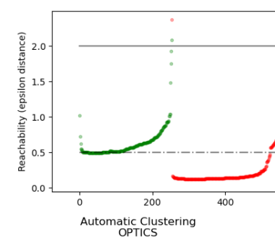
The reachability distances generated by OPTICS allow for variable density extraction of clusters within a single data set. As shown in the above plot, combining reachability distances and data set ordering_ produces a reachability plot, where point density is represented on the Y-axis, and points are ordered such that nearby points are adjacent. ‘Cutting’ the reachability plot at a single value produces DBSCAN like results; all points above the ‘cut’ are classified as noise, and each time that there is a break when reading from left to right signifies a new cluster. The default cluster extraction with OPTICS looks at the steep slopes within the graph to find clusters, and the user can define what counts as a steep slope using the parameter xi. There are also other possibilities for analysis on the graph itself, such as generating hierarchical representations of the data through reachability-plot dendrograms, and the hierarchy of clusters detected by the algorithm can be accessed through the cluster_hierarchy_ parameter. The plot above has been color-coded so that cluster colors in planar space match the linear segment clusters of the reachability plot. Note that the blue and red clusters are adjacent in the reachability plot, and can be hierarchically represented as children of a larger parent cluster.

Examples:  Demo of OPTICS clustering algorithm

Comparison with DBSCAN:

The results from OPTICS cluster_optics_dbscan method and DBSCAN are very similar, but not always identical; specifically, labeling of periphery and noise points. This is in part because the first samples of each dense area processed by OPTICS have a large reachability value while being close to other points in their area, and will thus sometimes be marked as noise rather than periphery. This affects adjacent points when they are considered as candidates for being marked as either periphery or noise.

Note that for any single value of eps, DBSCAN will tend to have a shorter run time than OPTICS; however, for repeated runs at varying eps values, a single run of OPTICS may require less cumulative runtime than DBSCAN. It is also important to note that OPTICS’ output is close to DBSCAN’s only if eps and max_eps are close.

Computational Complexity:

Spatial indexing trees are used to avoid calculating the full distance matrix, and allow for efficient memory usage on large sets of samples. Different distance metrics can be supplied via the metric keyword.

For large datasets, similar (but not identical) results can be obtained via HDBSCAN. The HDBSCAN implementation is multithreaded, and has better algorithmic runtime complexity than OPTICS, at the cost of worse memory scaling. For extremely large datasets that exhaust system memory using HDBSCAN, OPTICS will maintain n (as opposed to n2) memory scaling; however, tuning of the max_eps parameter will likely need to be used to give a solution in a reasonable amount of wall time.

References:

• “OPTICS: ordering points to identify the clustering structure.” Ankerst, Mihael, Markus M. Breunig, Hans-Peter Kriegel, and Jörg Sander. In ACM Sigmod Record, vol. 28, no. 2, pp. 49-60. ACM, 1999.