Quoted from: https://people.cs.umass.edu/~mccallum/courses/gm2011/02-bn-rep.pdf

Naive Bayes is a simple technique for constructing classifiers: models that assign class labels to problem instances, represented as vectors of feature values, where the class labels are drawn from some finite set. There is not a single algorithm for training such classifiers, but a family of algorithms based on a common principle: all naive Bayes classifiers assume that the value of a particular feature is independent of the value of any other feature, given the class variable. For example, a fruit may be considered to be an apple if it is red, round, and about 10 cm in diameter. A naive Bayes classifier considers each of these features to contribute independently to the probability that this fruit is an apple, regardless of any possible correlations between the color, roundness, and diameter features.

For some types of probability models, naive Bayes classifiers can be trained very efficiently in a supervised learning setting. In many practical applications, parameter estimation for naive Bayes models uses the method of maximum likelihood; in other words, one can work with the naive Bayes model without accepting Bayesian probability or using any Bayesian methods.

Despite their naive design and apparently oversimplified assumptions, naive Bayes classifiers have worked quite well in many complex real-world situations. In 2004, an analysis of the Bayesian classification problem showed that there are sound theoretical reasons for the apparently implausible efficacy of naive Bayes classifiers. Still, a comprehensive comparison with other classification algorithms in 2006 showed that Bayes classification is outperformed by other approaches, such as boosted trees or random forests.

An advantage of naive Bayes is that it only requires a small number of training data to estimate the parameters necessary for classification.

Abstractly, naïve Bayes is a conditional probability model: given a problem instance to be classified, represented by a vector {\displaystyle \mathbf {x} =(x_{1},\ldots ,x_{n})} representing some n features (independent variables), it assigns to this instance probabilities

{\displaystyle p(C_{k}\mid x_{1},\ldots ,x_{n})\,}

for each of K possible outcomes or classes {\displaystyle C_{k}}.

The problem with the above formulation is that if the number of features n is large or if a feature can take on a large number of values, then basing such a model on probability tables is infeasible. We therefore reformulate the model to make it more tractable. Using Bayes' theorem, the conditional probability can be decomposed as

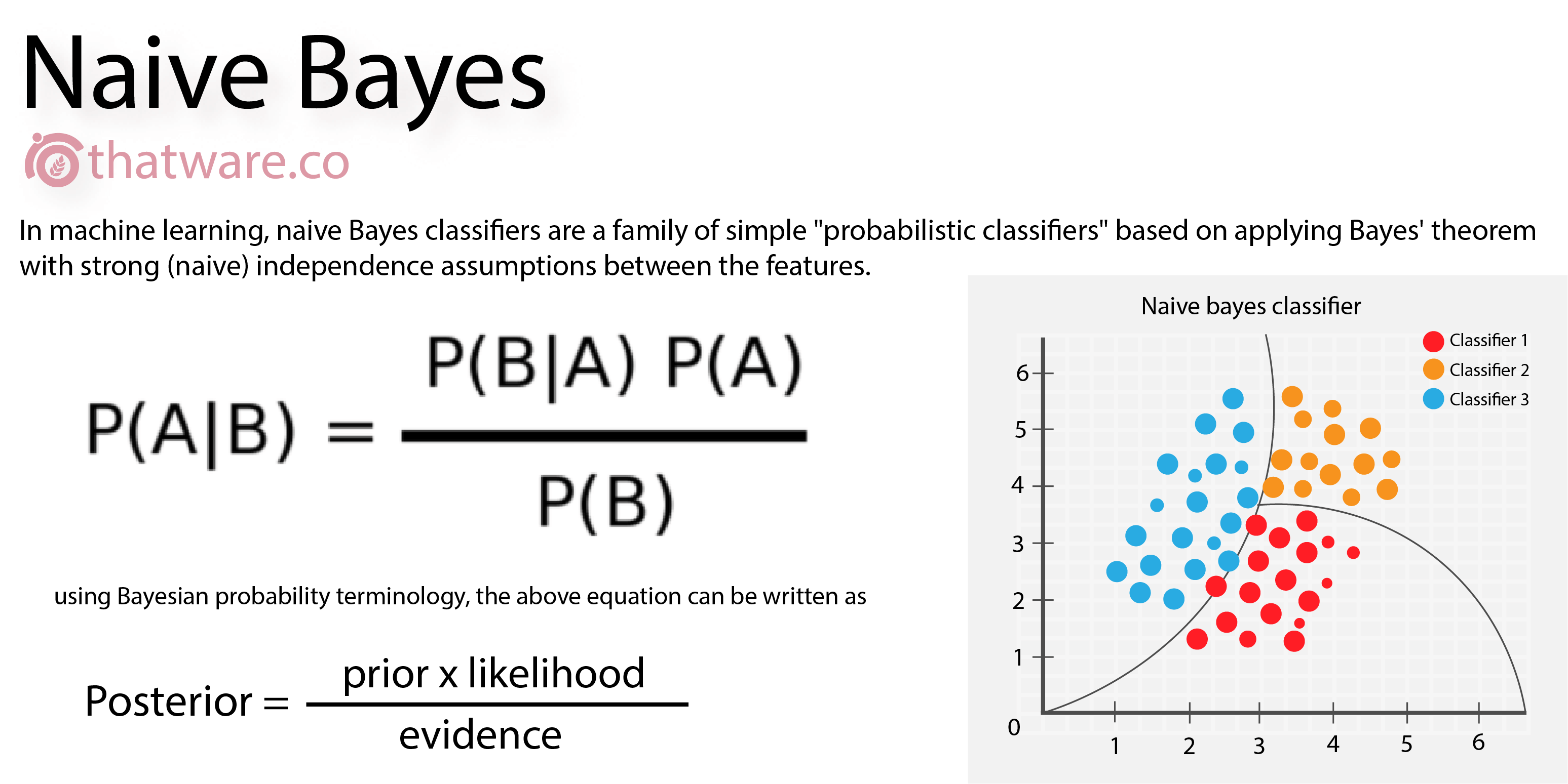
{\displaystyle p(C_{k}\mid \mathbf {x} )={\frac {p(C_{k})\ p(\mathbf {x} \mid C_{k})}{p(\mathbf {x} )}}\,}

In plain English, using Bayesian probability terminology, the above equation can be written as

{\displaystyle {\text{posterior}}={\frac {{\text{prior}}\times {\text{likelihood}}}{\text{evidence}}}\,}

In practice, there is interest only in the numerator of that fraction, because the denominator does not depend on {\displaystyle C} and the values of the features {\displaystyle x_{i}} are given, so that the denominator is effectively constant. The numerator is equivalent to the joint probability model

{\displaystyle p(C_{k},x_{1},\ldots ,x_{n})\,}

which can be rewritten as follows, using the chain rule for repeated applications of the definition of conditional probability:

{\displaystyle {\begin{aligned}p(C_{k},x_{1},\ldots ,x_{n})&=p(x_{1},\ldots ,x_{n},C_{k})\\&=p(x_{1}\mid x_{2},\ldots ,x_{n},C_{k})\ p(x_{2},\ldots ,x_{n},C_{k})\\&=p(x_{1}\mid x_{2},\ldots ,x_{n},C_{k})\ p(x_{2}\mid x_{3},\ldots ,x_{n},C_{k})\ p(x_{3},\ldots ,x_{n},C_{k})\\&=\cdots \\&=p(x_{1}\mid x_{2},\ldots ,x_{n},C_{k})\ p(x_{2}\mid x_{3},\ldots ,x_{n},C_{k})\cdots p(x_{n-1}\mid x_{n},C_{k})\ p(x_{n}\mid C_{k})\ p(C_{k})\\\end{aligned}}}

Now the "naïve" conditional independence assumptions come into play: assume that all features in {\displaystyle \mathbf {x} } are mutually independent, conditional on the category {\displaystyle C_{k}}. Under this assumption,

{\displaystyle p(x_{i}\mid x_{i+1},\ldots ,x_{n},C_{k})=p(x_{i}\mid C_{k})\,}.

Thus, the joint model can be expressed as

{\displaystyle {\begin{aligned}p(C_{k}\mid x_{1},\ldots ,x_{n})&\varpropto p(C_{k},x_{1},\ldots ,x_{n})\\&\varpropto p(C_{k})\ p(x_{1}\mid C_{k})\ p(x_{2}\mid C_{k})\ p(x_{3}\mid C_{k})\ \cdots \\&\varpropto p(C_{k})\prod _{i=1}^{n}p(x_{i}\mid C_{k})\,,\end{aligned}}}

where {\displaystyle \varpropto } denotes proportionality.

This means that under the above independence assumptions, the conditional distribution over the class variable {\displaystyle C} is:

{\displaystyle p(C_{k}\mid x_{1},\ldots ,x_{n})={\frac {1}{Z}}p(C_{k})\prod _{i=1}^{n}p(x_{i}\mid C_{k})}

where the evidence {\displaystyle Z=p(\mathbf {x} )=\sum _{k}p(C_{k})\ p(\mathbf {x} \mid C_{k})} is a scaling factor dependent only on {\displaystyle x_{1},\ldots ,x_{n}}, that is, a constant if the values of the feature variables are known.

The discussion so far has derived the independent feature model, that is, the naïve Bayes probability model. The naïve Bayes classifier combines this model with a decision rule. One common rule is to pick the hypothesis that is most probable; this is known as the maximum a posteriori or MAP decision rule. The corresponding classifier, a Bayes classifier, is the function that assigns a class label {\displaystyle {\hat {y}}=C_{k}} for some k as follows:

{\displaystyle {\hat {y}}={\underset {k\in \{1,\ldots ,K\}}{\operatorname {argmax} }}\ p(C_{k})\displaystyle \prod _{i=1}^{n}p(x_{i}\mid C_{k}).}