1 The response function of NPP to disturbances 

    The stand age distribution A(y, i ) can be determined using a Weibull distribution:

where q is the total fire and insect occurrence frequency, is the gamma function, and s is the shape parameter (Kasischke et al., 1995). We further assume that only mature forests are harvested. At y=0 (i.e. for areas disturbed and yet to regenerate), A(0, i ) was the difference between the disturbed and planted areas in previous n years, where n is the average age that a forest may need to start to regenerate. For example, n=5 for Canada’s forests, with a range of 1–10 years (Bunce, 1989). For each subsequent year, A(y, i ) is calculated by increasing the age by one year for not disturbed forest areas, returning the age to zero for newly disturbed forest areas, and entering age one for previously disturbed forest areas which at that time begin to regenerate. In this study, all areas are treated equally, and no spatial detail is involved. With the calculated A(y, i ) and F_NPP(y), the overall effect of disturbances on NPP is then given by

2 The response function of NPP to non-disturbances

    For C₃ plants, which include all Canada’s forests species, the instantaneous  photosynthesis rate of a single leaf p is limited by the minimum of the two values (Farquhar et al., 1980; Bonan,1995; Luo et al., 1996):

where p₁ and p₂ are leaf gross photosynthesis limited by electron transport and rubisco activity, respectively. The values of J, V_m, c_i, , and k_co in Eq. (4) are given by (Sellers et al., 1992; Bonan,1995):

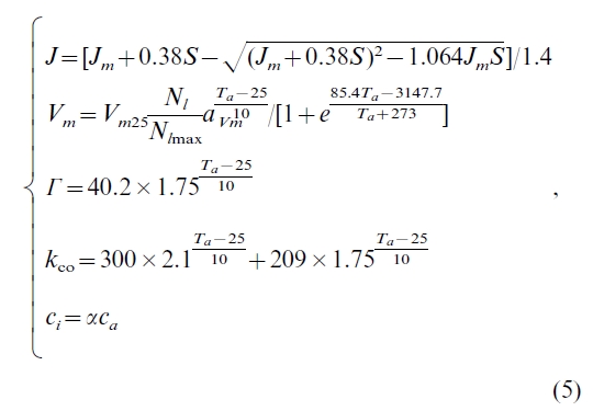
J_m=[J_m25(N_l/N_lmax)a_jm^(T_a-25)/10]/[1+exp((85.4T_a-3147.7)/(T_a+273))].The meanings of

other terms are listed in Notation. Eq. (5) shows that p is affected by climatic variables (i.e. T_a, S, and h_r) and atmospheric variables (i.e. c_a and N deposition). The effect of N deposition on p is incorporated through N_l/N_lmax (see details in Section 3).

    The area-averaged annual gross photosynthesis rate of a forest region in year i, P(i ), is then given by integrating p for all leaves (x) over the whole forest region (y) and time periods during the year (t)

    There are many ways to carry out this integration for all leaves in a stand (Norman, 1993). One way, simple yet effective, is to stratify a canopy into sunlit and shaded leaves (Norman, 1993), since T_a, c_a, and h_r are more or less the same for all leaves in a canopy because canopy air is often well mixed during daytime. This stratification is essential because irradiation changes greatly for different leaves depending on their positions relative to the sun, resulting in different J values for different leaves in the canopy. With this stratification and canopy radiation models (Black et al., 1991; Chen et al., 1999a), we calculate the instantaneous canopy photosynthesis rate, p_can, by the minimum of

where L_sun is the sunlit leaf area index, given by, whereis the gap fraction at the view zenith angle , calculated as (Nilson, 1971; Chen et al.,1997). The shaded leaf area index, Lshad, thus equals the difference of total leaf area index L_t and L_sun. Assuming no significant changes in morphology of leaves occurred since the industrialization, we can calculate the change in area-averaged L_t in year i by

The values of J for sunlit leaves and shaded leaves, J_sun and J_shad, are calculated by replacing S in Eq. (5) with S_sun and S_shad respectively, where S_sun and S_shad are calculated following Black et al. (1991) and Chen et al. (1999a). 

    Assuming f_p is the fraction of canopy photosynthesis limited by P_can1, we calculate the canopy photosynthesis rate over the time period by

    With p_can, we reduce Eq. (6) to

    While it is theoretically possible to calculate P(i) for each year since the industrialization, such an operation is practically limited by data availability. An alternative is to calculate P(i) only for a recent year for which quality data are available, and to determine P(i) in other years using a relationship between the interannual relative change in P(i),(dP(i)/[P(i)di]), and the external forcing factors. Differentiating Eq. (10) gives

    where term I represents the effect on dP(i)/di caused by changes in p_can(y, t), while term II and III represent, respectively, the effects caused by changes in forest cover area and growing season length (l_g). The value of dp_can(y, t) is given by differentiating Eq. (9):

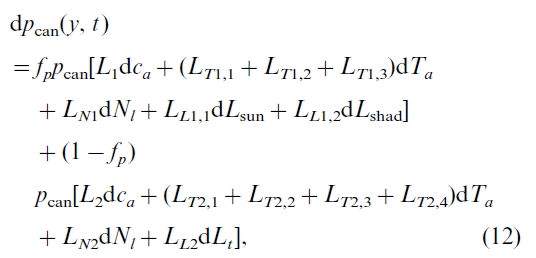where L₁, L₂, L_T1,1, L_T1,2, L_T1,3, L_N1, L_L1,1, L_L1,2,L_T2,1, L_T2,2, L_T2,3, L_T2,4, L_N2, and L_L2 are coefficients for the effects of CO₂ fertilization, climate variability, N availability, and leaf area changes (see Appendix A). Due to the lack of historical data about changes in h_r, S_sun, and S_shad since industrialization, we omit their impacts in this study. All these L terms (shortened as L_x) and pcan vary diurnally and seasonally as well as between locations. Due to the covariance between L_x and pcan, L_x cannot be factored out of the two-dimension integration in Eq. (11). To carry out this integration, detailed data for L_x and p_can are required. In reality, this is not feasible, especially for the long historical periods in this study. To avoid this difficulty, we use a 3-step spatial and temporal scaling algorithm: (1) To replace the integration by a discrete summation; (2) To estimate the discrete summation using the correlation coefficient, r, between the two variables L_x and p_can, namely,

where n is the number of data points in terms of both time periods and spatial locations, is the spatial and temporal assemble average of L_x in year i, and s is the standard deviation; and (3) To introduce a conversion coefficient,,that gives

, whereis calculated using annual mean values of climate,

N availability, and CO2 concentration. Using this algorithm, we express term I as follows:

    Term II in Eq. (11) is the effect of the change in forest area on the total photosynthesis. Since we consider only the existing forests, and LUC effects are outside the scope of this study. The changes in forest area due to disturbances are considered in Section 1.

    Term III in Eq. (11) is the result of growing season length changes, i.e.

    This term can be very important at high latitudes where the growing season is short and air temperature increased at a higher rate than that at low and middle latitudes (Frolking, 1997; Chen et al., 1999b). Inserting Eqs. (13) and (14) into Eq. (11), we calculate the interannual relative change in P(i ) by

    So far, we have considered only gross photosynthesis rate P(i ). NPP is only about 25–60% of P(i ), dependent on plant species, because a large part of P(i ) is consumed by autotrophic respiration (Ryan et al., 1997). Yet, the ratio of NPP to P(i ) is conservative with climate change and N status (Ryan et al., 1997), so that

From Eq. (1) and Eqs. (15) and (16), the effects of non-disturbance factors on NPP can then be calculated as

3 N cycle and leaf N content

    The total available N in the soils in year i, N_av,s(i ), is the sum of atmospheric N deposition

N_dep(i ), biotic N fixation N_fix(i ), and net N mineralization N_min(i )

    We use measured N_dep(i ) values (Ro et al., 1995). The value of N_fix(i ) is calculated based on the studies of Van Cleve and Alexander (1981), Parton et al. (1987), and Chapin and Bledsoe (1992) (see detail in Chen et al., 2000b). Net N mineralization is stochastically related to the C cycle through the C:N ratios and is calculated by:

    This equation follows the same principle as that of Townsend et al. (1996) and Holland et al. (1997), but differs in two aspects. One is that additional soil C pools are included in this equation. The second aspect is that we allow C/N ratios of biomass and soil C pools to vary, based on recent experimental findings. Many recent studies revealed that when grown in higher CO₂, plant issues (including green leaves) had consistently lower N concentration (e.g. Curtis et al., 1995). Yet leaf litter quality is essentially the same under different CO₂ levels because N is withdrawn prior to leaf senescence (O’Neill, 1994). In contrast, N in fine roots is not mobilized prior to senescence (Nambiar, 1987), and the C/N ratio was found to be much higher in fine roots grown under higher CO₂ environments (Norby, 1994). Experimental evidence also showed that C/N ratios of soil C pools vary from year to year (Schimel et al., 1994), and vary at different N and CO₂ levels (Pregitzer et al., 1995). Some recent models (e.g. Schimel et al., 1996; Comins, 1997) have incorporated these experimental findings of varying C/N ratios. In this study, we calculate a C/N ratio for each of the biomass and soil C pools as the ratio of total C content to total N content of the C pool in the year of concern.

    Due to N loss as a result of wildfire, harvest, gas emission, and leaching, only a fraction of N_av,s(i ) will be taken up by the plants. The value of N_up(i ) can be determined through solving three related equations: (1) N_av,s(i )=N_up(i )+N_loss(i );(2) a Michaelis–Menten relationship between N_up(i ) and the inorganic N concentration in the soil (Rastetter et al., 1991; Hudson et al., 1994); and (3) a linear relationship between N_loss(i ) and the inorganic N concentration in the soil. The solution for N_up(i ) is given by:

where the maximum uptake capacity Nup,max(i ) is given by b1[C_fr(i )/C_fr(0)] [CN_fr(i)/CN_fr(0)]-Q_10,Nup^{(T_s (i )-T_s (0))/10}, b₁ and b₂ are constants determined by equaling N input into and export from the forest ecosystems during the pre-industrial periods. In addition to the N_up(i ), the N transferred from senesced leaves in year i-1, N_tr(i ), also contributes to the total available N in plants in year i, N_av,p(i ).

    We use the same coefficients partitioning N_av,p to green leaf, fine roots, wood, and coarse roots in year i as in year i-1 because there is no evidence that these coefficients vary in one way or another. Equations for calculating C/N ratio of green leaf, fine roots, wood, coarse roots, fine structure detritus, coarse structure detritus, and slow soil C are given in Appendix A. The C/N ratios of microbe, metabolic detritus, passive soil C, and charcoal are assumed to be constant. With the known values of CN_l(i ) and Lt(i ), and Cl(i ), the mean leaf N content per unit leaf area at year i, Nl(i ), can be calculated as follows

where the value of Nl(i ) is constrained to Nlmax(i ). Since the relationship between age and NPP is empirically pre-determined, the interactions between changes in NPP caused by age class shift and N cycle have already been included in the age–NPP relationship. Therefore, the value of Nl(i ) is calculated after considering only the climatic and atmospheric changes.

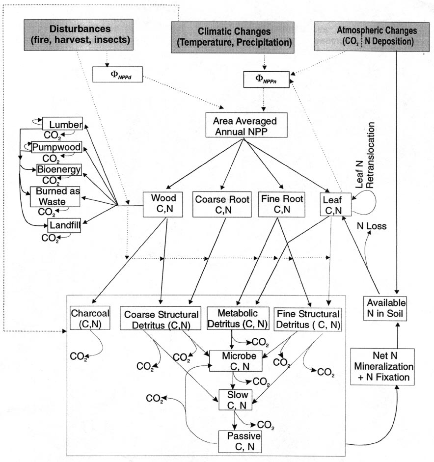
4 C cycle

    The change in the size of each C pool in InTEC is described by the first-order rate kinetics (Paul and Clark, 1996)

    where Input(i ) is a fraction of NPP transferred to biomass C pools or a fraction of upstream C pools to soil and forest product C pools. It is important to note that if inventory-based C_x(i ) and estimated NPP are used, which can only be measured or estimated with limited accuracy, a large error can be introduced in , which is usually much smaller than NPP or k_x(i )Cx(i ) in a given year. To avoid this error, we rearrange Eq. (22) by taking Cx(i ) as Cx(i-1)+, so that

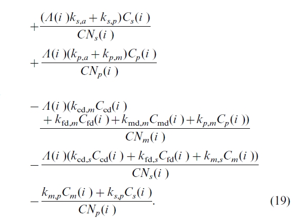
    To calculate Cx(i-1), Cx(i-2) and NPP(i-1) are needed. This procedure continues, until the pre-industrial period is reached during which we assume under the mean disturbance rates and climatic and atmospheric conditions. This procedure shows that depends on historical changes in disturbance rates and climatic conditions over the entire time period since the industrialization. Following this procedure, the changes in biomass, soil, and forest products C pools are calculated by subtracting C output terms (i.e. transfer to downstream pools, and fire emission, oxidation, and respiration to the  atmosphere) from the input terms (i.e. fraction of NPP partitioned to the C pool concerned, and C transfer from upstream pools). Farquhar and Henry (1997) estimated that -10% of remaining wood after burning will become charcoal instead of C_cd, and we adopt this percentage in this study. The value of Fm(i ) affects the partitioning of leave and fine roots litter to detritus C pools, and is given by F_m(i )=0.85-0.018LN(i ) (Schimel et al., 1996).Equations for calculating changes in biomass, soil, and forest products C pools are given in Appendix A. For the five product pools, the changes in the sizes of lumber (), pulp-wood (),and landfills () C pools are calculated also using the first-order rate kinetics in the same way as for ecosystem C pools, while the bio-energy and burned-as-waste release C within a year.

    Summation of these C pool changes gives the area-averaged annual C balance or NBP in year i. The cumulative change in each of these C pools is obtained by integrating the change since the industrialization.